BaseAttentive: Hybrid vs Transformer Architectures
This notebook compares the two main architectural choices in BaseAttentive:
Hybrid: Multi-scale LSTM + Attention (captures temporal patterns + global context)
Transformer: Pure self-attention (global context only)
[1]:
# ── v2.2.0 Backend Setup ─────────────────────────────────────────────────────
# BASE_ATTENTIVE_BACKEND must be set *before* importing base_attentive.
# Choose your installed backend: "tensorflow" | "torch" | "jax" | "auto"
import os
os.environ.setdefault("BASE_ATTENTIVE_BACKEND", "tensorflow")
os.environ.setdefault("KERAS_BACKEND", os.environ["BASE_ATTENTIVE_BACKEND"])
import keras  # initialise Keras 3 backend before base_attentive
BACKEND = os.environ["BASE_ATTENTIVE_BACKEND"]
print(f"Backend: {BACKEND}")
Backend: tensorflow
[2]:
from base_attentive import BaseAttentive
Common Configuration
[3]:
# Shared parameters
STATIC_DIM = 4
DYNAMIC_DIM = 8
FUTURE_DIM = 6
OUTPUT_DIM = 1
FORECAST_HORIZON = 24

shared_params = {
    "static_input_dim": STATIC_DIM,
    "dynamic_input_dim": DYNAMIC_DIM,
    "future_input_dim": FUTURE_DIM,
    "output_dim": OUTPUT_DIM,
    "forecast_horizon": FORECAST_HORIZON,
    "embed_dim": 32,
    "attention_units": 64,
    "num_heads": 8,
    "dropout_rate": 0.1,
}

print("✅ Shared parameters defined")
✅ Shared parameters defined
Model 1: Hybrid Architecture (LSTM + Attention)
Characteristics:
Multi-scale LSTM for hierarchical temporal feature extraction
Attention mechanisms for global context
Best for: Complex temporal patterns, shorter sequences
Pros: Captures temporal correlations well
Cons: Slower training/inference
[4]:
# Hybrid model: LSTM + Attention
hybrid_config = {
    **shared_params,
    "objective": "hybrid",  # Uses LSTM encoder
    "name": "HybridModel",
}

hybrid_model = BaseAttentive(**hybrid_config)

print("🔧 Hybrid Model Configuration:")
print(f"  Objective: {hybrid_model.objective}")
print(f"  LSTM Units: {hybrid_model.lstm_units}")
print(f"  Scales: {hybrid_model.scales}")
print(f"  Mode: {hybrid_model.mode}")
D:\projects\base-attentive\src\base_attentive\core\base_attentive.py:148: DeprecatedParameterWarning: BaseAttentive: 'static_input_dim' is deprecated since 2.1.0 and will be removed in 3.0.0. Use 'static_dim' instead.
  resolved = resolve_deprecated_kwargs(
D:\projects\base-attentive\src\base_attentive\core\base_attentive.py:148: DeprecatedParameterWarning: BaseAttentive: 'dynamic_input_dim' is deprecated since 2.1.0 and will be removed in 3.0.0. Use 'dynamic_dim' instead.
  resolved = resolve_deprecated_kwargs(
D:\projects\base-attentive\src\base_attentive\core\base_attentive.py:148: DeprecatedParameterWarning: BaseAttentive: 'future_input_dim' is deprecated since 2.1.0 and will be removed in 3.0.0. Use 'future_dim' instead.
  resolved = resolve_deprecated_kwargs(
🔧 Hybrid Model Configuration:
  Objective: hybrid
  LSTM Units: 64
  Scales: None
  Mode: None
Model 2: Transformer Architecture (Pure Attention)
Characteristics:
Pure self-attention stack, no recurrence
Parallel computation across sequence
Best for: Long sequences, global dependencies
Pros: Faster, captures long-range dependencies
Cons: May miss local temporal patterns
[5]:
# Transformer model: Pure Attention
transformer_config = {
    **shared_params,
    "objective": "transformer",  # Pure attention encoder
    "num_encoder_layers": 2,  # Number of attention blocks
    "name": "TransformerModel",
}

transformer_model = BaseAttentive(**transformer_config)

print("🔧 Transformer Model Configuration:")
print(f"  Objective: {transformer_model.objective}")
print(
    f"  Encoder Layers: {transformer_model.num_encoder_layers}"
)
print(
    f"  Attention Units: {transformer_model.attention_units}"
)
print(f"  Mode: {transformer_model.mode}")
🔧 Transformer Model Configuration:
  Objective: transformer
  Encoder Layers: 2
  Attention Units: 64
  Mode: None
Comparison Table
[6]:
import pandas as pd

comparison_data = {
    "Aspect": [
        "Encoder Type",
        "Speed (Training)",
        "Speed (Inference)",
        "Temporal Patterns",
        "Long-Range Dependencies",
        "Memory Usage",
        "Best For",
        "Sequence Length",
    ],
    "Hybrid (LSTM+Attn)": [
        "Multi-scale LSTM",
        "Slower",
        "Slower",
        "Excellent",
        "Good",
        "Higher",
        "Complex temporal data",
        "Short to medium",
    ],
    "Transformer (Pure Attn)": [
        "Self-Attention Stack",
        "Faster",
        "Faster",
        "Good",
        "Excellent",
        "Lower",
        "Long sequences",
        "Long",
    ],
}

df = pd.DataFrame(comparison_data)
print(df.to_string(index=False))
                 Aspect    Hybrid (LSTM+Attn) Transformer (Pure Attn)
           Encoder Type      Multi-scale LSTM    Self-Attention Stack
       Speed (Training)                Slower                  Faster
      Speed (Inference)                Slower                  Faster
      Temporal Patterns             Excellent                    Good
Long-Range Dependencies                  Good               Excellent
           Memory Usage                Higher                   Lower
               Best For Complex temporal data          Long sequences
        Sequence Length       Short to medium                    Long
Advanced Configuration: Using architecture_config
You can also use architecture_config for fine-grained control.
[7]:
# Advanced configuration with architecture_config
custom_architecture = {
    "encoder_type": "transformer",
    "decoder_attention_stack": [
        "cross",
        "hierarchical",
    ],  # Skip memory attention
    "feature_processing": "dense",  # Use dense instead of VSN
}

custom_model = BaseAttentive(
    **shared_params,
    architecture_config=custom_architecture,
    name="CustomModel",
)

print("🎨 Custom Architecture Configuration:")
print(
    f"  Encoder Type: {custom_model.architecture_config.get('encoder_type')}"
)
print(
    f"  Attention Stack: {custom_model.architecture_config.get('decoder_attention_stack')}"
)
print(
    f"  Feature Processing: {custom_model.architecture_config.get('feature_processing')}"
)
🎨 Custom Architecture Configuration:
  Encoder Type: transformer
  Attention Stack: ['cross', 'hierarchical']
  Feature Processing: dense
D:\projects\base-attentive\src\base_attentive\core\base_attentive.py:148: DeprecatedParameterWarning: BaseAttentive: 'static_input_dim' is deprecated since 2.1.0 and will be removed in 3.0.0. Use 'static_dim' instead.
  resolved = resolve_deprecated_kwargs(
D:\projects\base-attentive\src\base_attentive\core\base_attentive.py:148: DeprecatedParameterWarning: BaseAttentive: 'dynamic_input_dim' is deprecated since 2.1.0 and will be removed in 3.0.0. Use 'dynamic_dim' instead.
  resolved = resolve_deprecated_kwargs(
D:\projects\base-attentive\src\base_attentive\core\base_attentive.py:148: DeprecatedParameterWarning: BaseAttentive: 'future_input_dim' is deprecated since 2.1.0 and will be removed in 3.0.0. Use 'future_dim' instead.
  resolved = resolve_deprecated_kwargs(
Training Both Architectures
Train Hybrid and Transformer models on identical synthetic data to compare convergence and forecast quality.
[8]:
import numpy as np
import keras

np.random.seed(42)
N, T, H = 64, 20, 24  # samples, lookback, horizon

# ── Synthetic sine-wave data ──────────────────────────────────────────
t_past   = np.linspace(0, 4*np.pi, T)
t_future = np.linspace(4*np.pi, 6*np.pi, H)
noise    = lambda s: np.random.randn(*s).astype('float32') * 0.15

static_d  = np.random.randn(N, STATIC_DIM ).astype('float32')
dynamic_d = (np.tile(np.sin(t_past),   (N, 1))[:, :, None]
             * np.random.rand(N, 1, DYNAMIC_DIM) + noise((N, T, DYNAMIC_DIM)))
future_d  = (np.tile(np.cos(t_future), (N, 1))[:, :, None]
             * np.random.rand(N, 1, FUTURE_DIM)  + noise((N, H, FUTURE_DIM)))
target_d  = (np.tile(np.sin(t_future), (N, 1))[:, :, None]
             + noise((N, H, OUTPUT_DIM))).astype('float32')

print(f'Data — static:{static_d.shape}  dynamic:{dynamic_d.shape}  future:{future_d.shape}  target:{target_d.shape}')
Data — static:(64, 4) dynamic:(64, 20, 8) future:(64, 24, 6) target:(64, 24, 1)
[9]:
def compile_and_train(model, label, epochs=12):
    _ = model([static_d, dynamic_d, future_d])  # build weights
    model.compile(optimizer=keras.optimizers.Adam(1e-3), loss='mse', metrics=['mae'])
    h = model.fit(
        [static_d, dynamic_d, future_d], target_d,
        epochs=epochs, batch_size=16, validation_split=0.2, verbose=0,
    )
    print(f'{label:30s}  train MSE={h.history["loss"][-1]:.4f}  val MSE={h.history["val_loss"][-1]:.4f}')
    return h

print('Training...')
h_hybrid      = compile_and_train(hybrid_model,      'Hybrid (LSTM + Attention)')
h_transformer = compile_and_train(transformer_model, 'Transformer (Pure Attention)')
print('Done.')
Training...
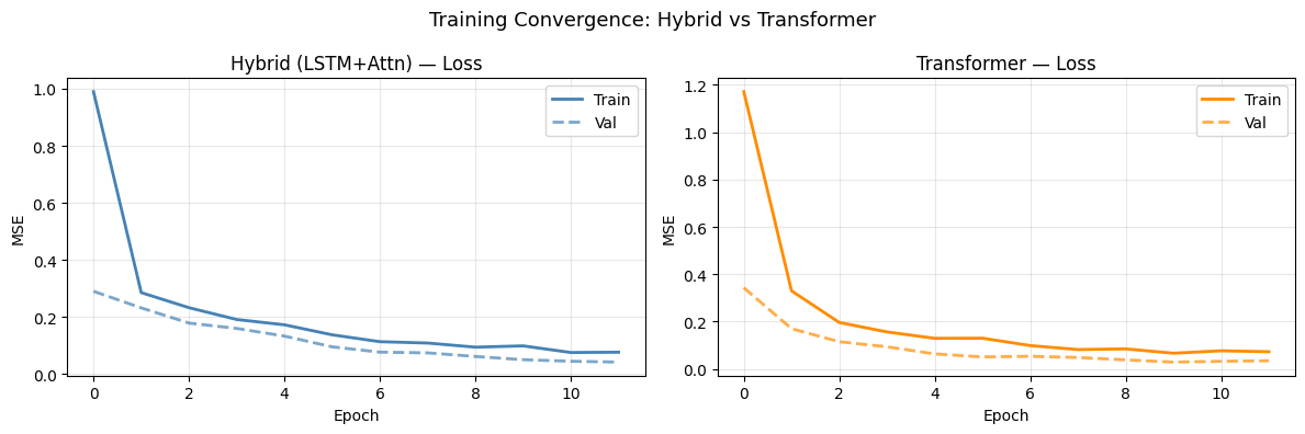
Hybrid (LSTM + Attention) train MSE=0.0763 val MSE=0.0417
Transformer (Pure Attention) train MSE=0.0725 val MSE=0.0344
Done.
Plot 1 — Training Loss Curves
Side-by-side convergence curves show which architecture reaches lower loss faster.
[10]:
import matplotlib.pyplot as plt

fig, axes = plt.subplots(1, 2, figsize=(12, 4))
for ax, h, label, color in zip(
    axes,
    [h_hybrid, h_transformer],
    ['Hybrid (LSTM+Attn)', 'Transformer'],
    ['steelblue', 'darkorange'],
):
    ax.plot(h.history['loss'],     label='Train', color=color,  linewidth=2)
    ax.plot(h.history['val_loss'], label='Val',   color=color,  linewidth=2, linestyle='--', alpha=0.7)
    ax.set_title(f'{label} — Loss', fontsize=12)
    ax.set_xlabel('Epoch')
    ax.set_ylabel('MSE')
    ax.legend()
    ax.grid(True, alpha=0.3)

plt.suptitle('Training Convergence: Hybrid vs Transformer', fontsize=13)
plt.tight_layout()
plt.show()
Plot 2 — Forecast vs Actual
Overlay both models’ predictions against the true target for the same test sample.
[11]:
# Predict with both models (use last 10 samples as 'test')
test_slice = slice(-10, None)
pred_h = hybrid_model.predict(
    [static_d[test_slice], dynamic_d[test_slice], future_d[test_slice]], verbose=0)
pred_t = transformer_model.predict(
    [static_d[test_slice], dynamic_d[test_slice], future_d[test_slice]], verbose=0)

sample = 0
steps  = np.arange(1, H + 1)

fig, ax = plt.subplots(figsize=(10, 4))
ax.plot(steps, target_d[test_slice][sample, :, 0],
        label='Actual',      color='black',      linewidth=2.5)
ax.plot(steps, pred_h[sample, :, 0],
        label='Hybrid',      color='steelblue',  linewidth=2, linestyle='--')
ax.plot(steps, pred_t[sample, :, 0],
        label='Transformer', color='darkorange', linewidth=2, linestyle=':')

ax.set_title('Forecast vs Actual — Hybrid vs Transformer', fontsize=13)
ax.set_xlabel('Forecast step')
ax.set_ylabel('Value')
ax.legend()
ax.grid(True, alpha=0.3)
plt.tight_layout()
plt.show()

print(f'Hybrid      MAE: {float(np.mean(np.abs(pred_h - target_d[test_slice]))):.4f}')
print(f'Transformer MAE: {float(np.mean(np.abs(pred_t - target_d[test_slice]))):.4f}')
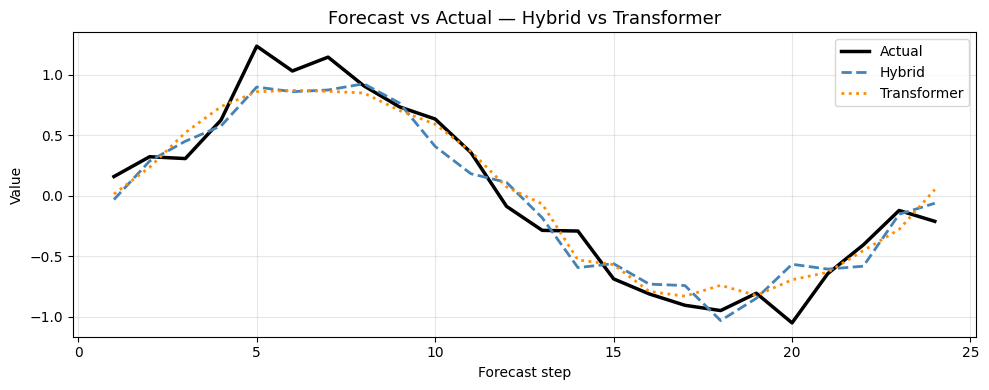
Hybrid      MAE: 0.1593
Transformer MAE: 0.1481
Recommendation
Use Hybrid when:
Your data has strong short-term temporal correlations
Sequences are short to medium length (< 50 steps)
You need to capture multi-scale temporal patterns
Use Transformer when:
Long-range dependencies are important
Sequences are long (> 100 steps)
You prioritize speed and have sufficient compute
Your data is mostly stationary with trend/seasonality