PADR-Net Flood Forecasting
Notebook goal: build, train, and interpret the new
PADRNetflood-forecasting application model. We create regional synthetic flood events for WAF, EAF, and SAF, train PADR-Net with a physics-aware loss, and evaluate depth forecasts, threshold skill, mass bias, and spatial-style interpretation maps.
This notebook is intentionally self-contained. The synthetic data are not meant to replace hydrodynamic simulation or observations; they are a compact teaching dataset that exposes the same API shape used with real forcing and flood-depth arrays.
[1]:
import os
import warnings

warnings.filterwarnings("ignore")

# PADR-Net currently provides TensorFlow and Torch backends.  The main
# tutorial uses TensorFlow because the training loop is compact and the
# same public PADRNet factory is used for both backends.
os.environ.setdefault("BASE_ATTENTIVE_BACKEND", "tensorflow")
os.environ.setdefault("KERAS_BACKEND", "tensorflow")

print("BASE_ATTENTIVE_BACKEND =", os.environ["BASE_ATTENTIVE_BACKEND"])
print("KERAS_BACKEND =", os.environ["KERAS_BACKEND"])
BASE_ATTENTIVE_BACKEND = tensorflow
KERAS_BACKEND = tensorflow
1. Imports and Reproducibility
The flood application exports the model factory, validated configuration, hydrological metrics, and backend-neutral physics helpers. The model output is a dictionary with three keys:
depth: multi-horizon flood depth forecast;exceedance_probability: smooth threshold-exceedance probability;features: latent event representation.
[2]:
from __future__ import annotations

import math
from dataclasses import dataclass

import matplotlib.pyplot as plt
import numpy as np
import tensorflow as tf

from base_attentive import PADRNet, PADRNetConfig
from base_attentive.applications.flood import (
    critical_success_index,
    delta_mass,
    exceedance_probability,
    linear_reservoir_response,
    mass_balance_residual,
    nash_sutcliffe_efficiency,
    true_skill_statistic,
)

np.random.seed(42)
tf.random.set_seed(42)
tf.get_logger().setLevel("ERROR")

plt.rcParams.update(
    {
        "figure.dpi": 120,
        "axes.spines.top": False,
        "axes.spines.right": False,
        "axes.grid": True,
        "grid.alpha": 0.25,
    }
)
2. Synthetic Regional Flood Events
We generate event hydrographs with a simple rainfall-storage response. Each region has a different response time, rainfall gain, basin area, slope, and imperviousness proxy. This gives PADR-Net a reason to use both dynamic sequences and static descriptors.
The split mimics a paper workflow: early years are used for training, intermediate years for validation, and later years for testing.
[3]:
@dataclass(frozen=True)
class RegionSpec:
    code: str
    name: str
    color: str
    tau: float
    gain: float
    area: float
    slope: float
    impervious: float
    storm_scale: float


REGIONS = [
    RegionSpec(
        "WAF", "West Africa", "#1f66b1", 28.0, 0.020,
        0.72, 0.36, 0.22, 1.15,
    ),
    RegionSpec(
        "EAF", "East Africa", "#f05a28", 20.0, 0.018,
        0.54, 0.52, 0.18, 1.00,
    ),
    RegionSpec(
        "SAF", "South Africa", "#2f8f3b", 34.0, 0.015,
        0.61, 0.31, 0.15, 0.92,
    ),
]

LOOKBACK = 48
HORIZON = 24
TOTAL_STEPS = LOOKBACK + HORIZON
INPUT_DIM = 8
STATIC_DIM = 3
FLOOD_THRESHOLD = 0.08


def rolling_mean(values: np.ndarray, window: int) -> np.ndarray:
    kernel = np.ones(window, dtype=float) / window
    return np.convolve(values, kernel, mode="same")


def make_storm(rng: np.random.Generator, spec: RegionSpec) -> np.ndarray:
    t = np.arange(TOTAL_STEPS)
    rain = rng.gamma(1.2, 0.12, TOTAL_STEPS)
    n_pulses = rng.integers(1, 4)
    for _ in range(n_pulses):
        center = rng.uniform(10, LOOKBACK + 8)
        width = rng.uniform(2.5, 8.0)
        height = rng.uniform(1.0, 4.0) * spec.storm_scale
        rain += height * np.exp(-0.5 * ((t - center) / width) ** 2)
    return np.maximum(rain, 0.0)


def make_event(
    rng: np.random.Generator,
    spec: RegionSpec,
    year: int,
) -> dict[str, np.ndarray | str | int]:
    rain = make_storm(rng, spec)
    depth = linear_reservoir_response(
        rain,
        tau=spec.tau,
        gain=spec.gain,
        initial_depth=rng.uniform(0.0, 0.01),
    )
    depth *= 8.0
    depth += 0.015 * np.sin(np.linspace(0, 2 * np.pi, TOTAL_STEPS))
    depth += rng.normal(0.0, 0.002, TOTAL_STEPS)
    depth = np.maximum(depth, 0.0)

    antecedent = rolling_mean(rain, 6)
    wetness = rolling_mean(rain, 18)
    response_proxy = linear_reservoir_response(
        rain,
        tau=max(8.0, spec.tau * 0.65),
        gain=spec.gain * 0.8,
    )
    hour = np.arange(TOTAL_STEPS) / 24.0
    seasonal = (year - 2001) / 23.0

    dynamic = np.column_stack(
        [
            rain,
            antecedent,
            wetness,
            response_proxy,
            np.sin(2 * np.pi * hour),
            np.cos(2 * np.pi * hour),
            np.full(TOTAL_STEPS, seasonal),
            np.gradient(rain),
        ]
    )
    static = np.array([spec.area, spec.slope, spec.impervious])
    return {
        "region": spec.code,
        "year": year,
        "x": dynamic[:LOOKBACK].astype("float32"),
        "static": static.astype("float32"),
        "y": depth[LOOKBACK:].astype("float32")[:, None],
        "rain_future": rain[LOOKBACK:].astype("float32")[:, None],
        "depth_full": depth.astype("float32"),
        "rain_full": rain.astype("float32"),
    }


def make_dataset(n_events: int = 720, seed: int = 13):
    rng = np.random.default_rng(seed)
    events = []
    years = rng.integers(2001, 2025, n_events)
    for year in years:
        spec = REGIONS[int(rng.integers(0, len(REGIONS)))]
        events.append(make_event(rng, spec, int(year)))
    return events


events = make_dataset()
print(f"events: {len(events)}")
print("first event keys:", sorted(events[0].keys()))
events: 720
first event keys: ['depth_full', 'rain_full', 'rain_future', 'region', 'static', 'x', 'y', 'year']
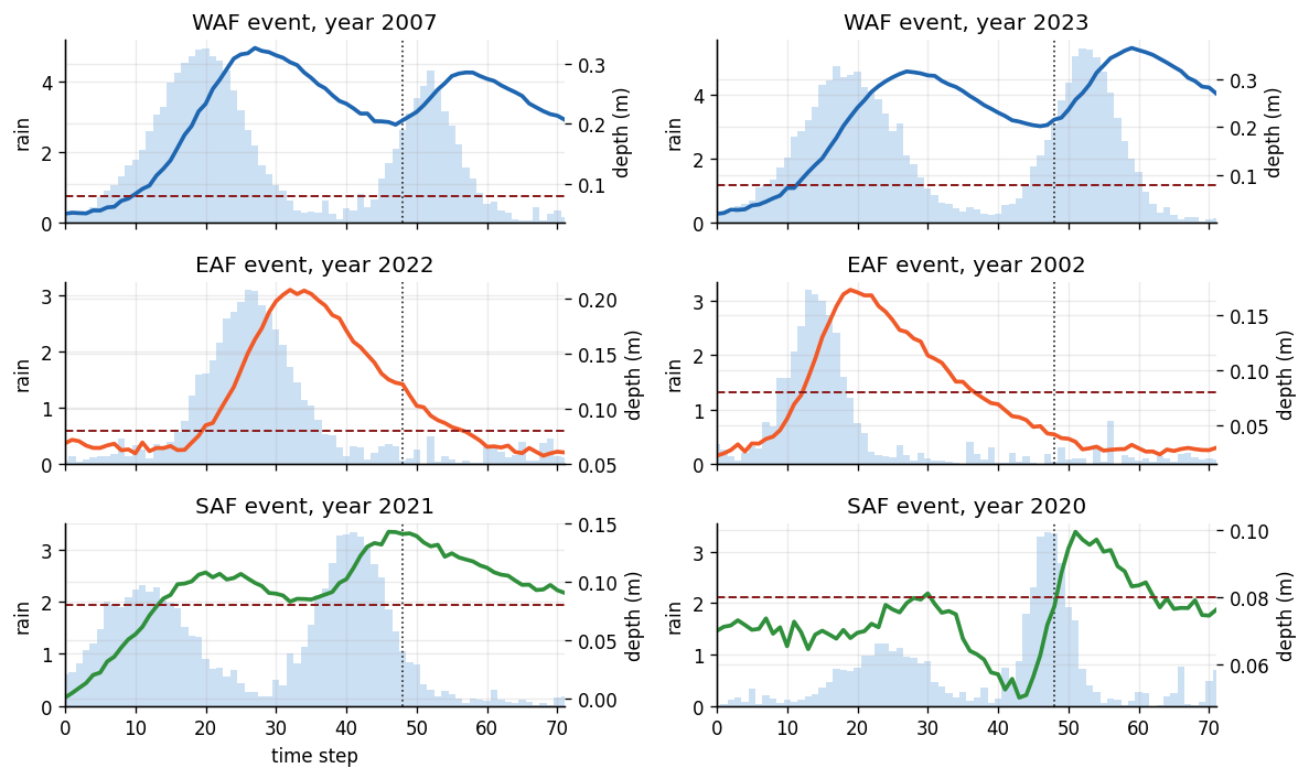
Visual check: rainfall and flood response
Before training a neural model, always inspect a few hydrographs. The vertical line marks the forecast origin. PADR-Net receives the left side and predicts the right side.
[4]:
def plot_event_examples(events, n_per_region=1):
    fig, axes = plt.subplots(3, n_per_region, figsize=(10, 6), sharex=True)
    axes = np.atleast_2d(axes)
    for row, spec in enumerate(REGIONS):
        region_events = [e for e in events if e["region"] == spec.code]
        for col, event in enumerate(region_events[:n_per_region]):
            ax = axes[row, col]
            t = np.arange(TOTAL_STEPS)
            ax2 = ax.twinx()
            ax.bar(
                t,
                event["rain_full"],
                color="#8fbce6",
                alpha=0.45,
                width=1.0,
                label="rainfall",
            )
            ax2.plot(
                t,
                event["depth_full"],
                color=spec.color,
                lw=2.2,
                label="depth",
            )
            ax2.axhline(
                FLOOD_THRESHOLD,
                color="#8b1e1e",
                lw=1.2,
                ls="--",
                label="threshold",
            )
            ax.axvline(LOOKBACK, color="#222", lw=1.0, ls=":")
            ax.set_title(f"{spec.code} event, year {event['year']}")
            ax.set_ylabel("rain")
            ax2.set_ylabel("depth (m)")
            ax.set_xlim(0, TOTAL_STEPS - 1)
    axes[-1, 0].set_xlabel("time step")
    fig.tight_layout()
    return fig

plot_event_examples(events, n_per_region=2)
plt.show()
3. Build Arrays and Temporal Splits
The arrays follow the PADR-Net input contract:
X:(batch, lookback, input_dim);S:(batch, static_dim);Y:(batch, forecast_horizon, 1);P_future:(batch, forecast_horizon, 1)for physics diagnostics.
[5]:
X = np.stack([e["x"] for e in events]).astype("float32")
S = np.stack([e["static"] for e in events]).astype("float32")
Y = np.stack([e["y"] for e in events]).astype("float32")
P_future = np.stack([e["rain_future"] for e in events]).astype("float32")
years = np.array([e["year"] for e in events])
regions = np.array([e["region"] for e in events])

train_idx = np.where(years <= 2018)[0]
val_idx = np.where((years >= 2019) & (years <= 2020))[0]
test_idx = np.where(years >= 2021)[0]

print("X:", X.shape, "S:", S.shape, "Y:", Y.shape)
print("train/val/test:", len(train_idx), len(val_idx), len(test_idx))

for spec in REGIONS:
    count = np.sum(regions == spec.code)
    print(f"{spec.code}: {count} events")
X: (720, 48, 8) S: (720, 3) Y: (720, 24, 1)
train/val/test: 541 56 123
WAF: 235 events
EAF: 217 events
SAF: 268 events
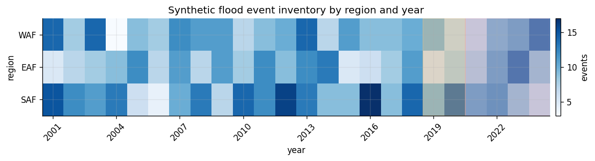
Regional inventory plot
This plot is not used by the model. It helps verify that all three regions are represented through time and that validation/test years are visible.
[6]:
def plot_event_inventory(years, regions):
    year_grid = np.arange(2001, 2025)
    counts = np.zeros((len(REGIONS), len(year_grid)), dtype=int)
    for i, spec in enumerate(REGIONS):
        for j, year in enumerate(year_grid):
            counts[i, j] = np.sum((regions == spec.code) & (years == year))

    fig, ax = plt.subplots(figsize=(11, 2.8))
    im = ax.imshow(counts, cmap="Blues", aspect="auto")
    ax.axvspan(2018.5 - 2001, 2020.5 - 2001, color="#f8c27c", alpha=0.35)
    ax.axvspan(2020.5 - 2001, 2024.5 - 2001, color="#ef9cae", alpha=0.28)
    ax.set_yticks(range(len(REGIONS)), [r.code for r in REGIONS])
    ax.set_xticks(range(0, len(year_grid), 3), year_grid[::3], rotation=45)
    ax.set_title("Synthetic flood event inventory by region and year")
    ax.set_xlabel("year")
    ax.set_ylabel("region")
    cbar = fig.colorbar(im, ax=ax, pad=0.01)
    cbar.set_label("events")
    fig.tight_layout()
    return fig

plot_event_inventory(years, regions)
plt.show()
4. Configure PADR-Net
The validated PADRNetConfig records the input dimensions, attention capacity, forecast horizon, threshold, and physics weights. The public PADRNet factory returns a backend-specific model while preserving the same API.
[7]:
config = PADRNetConfig(
    input_dim=INPUT_DIM,
    static_dim=STATIC_DIM,
    hidden_dim=48,
    num_heads=4,
    num_layers=2,
    forecast_horizon=HORIZON,
    dropout=0.05,
    lambda_physics=0.25,
    lambda_mass=0.05,
    lambda_smooth=0.01,
    flood_threshold=FLOOD_THRESHOLD,
    reservoir_tau=24.0,
)

model = PADRNet(config, backend="tensorflow")
outputs = model(tf.zeros((2, LOOKBACK, INPUT_DIM)), tf.zeros((2, STATIC_DIM)))

print(type(model).__name__)
for key, value in outputs.items():
    print(f"{key:24s}", tuple(value.shape))
TensorFlowPADRNet
depth                    (2, 24, 1)
exceedance_probability   (2, 24, 1)
features                 (2, 48)
5. Physics-Aware Training Loop
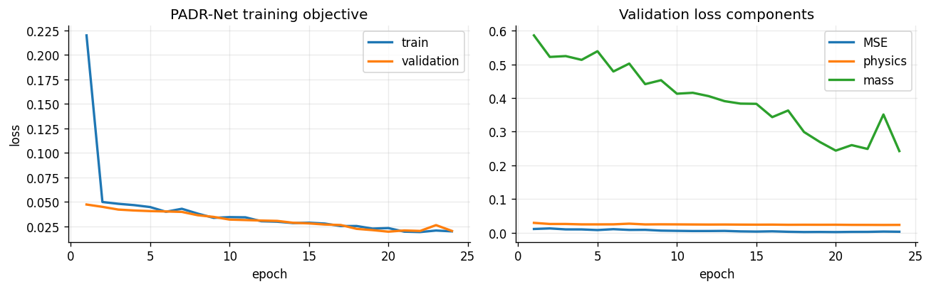
PADR-Net produces predictions; the training loop decides how to combine losses. Here we use:
\begin{align} \mathcal{L} = \mathcal{L}_{\mathrm{mse}} + \lambda_{\mathrm{phys}} \lVert r_t \rVert_2^2 + \lambda_{\mathrm{mass}} |\Delta M| + \lambda_{\mathrm{smooth}} \lVert \nabla_t \hat{h} \rVert_2^2. \end{align}
The residual is a simple rainfall-storage tendency. Real projects can replace it with a hydrodynamic operator, differentiable routing layer, or physics residual from a SWE/hydrological solver.
[8]:
BATCH_SIZE = 48
EPOCHS = 24


def make_tf_dataset(indices, shuffle=False):
    ds = tf.data.Dataset.from_tensor_slices(
        (X[indices], S[indices], Y[indices], P_future[indices])
    )
    if shuffle:
        ds = ds.shuffle(len(indices), seed=42, reshuffle_each_iteration=True)
    return ds.batch(BATCH_SIZE).prefetch(tf.data.AUTOTUNE)


train_ds = make_tf_dataset(train_idx, shuffle=True)
val_ds = make_tf_dataset(val_idx, shuffle=False)
test_ds = make_tf_dataset(test_idx, shuffle=False)

try:
    optimizer = tf.keras.optimizers.Adam(learning_rate=3e-3)
except (ImportError, ModuleNotFoundError):
    from tensorflow.python.keras.optimizer_v2.adam import Adam

    optimizer = Adam(learning_rate=3e-3)


def physics_terms(y_true, y_pred, rain_future, cfg, gain_proxy):
    pred = tf.squeeze(y_pred, axis=-1)
    true = tf.squeeze(y_true, axis=-1)
    rain = tf.squeeze(rain_future, axis=-1)

    mse = tf.reduce_mean(tf.square(true - pred))
    dh = pred[:, 1:] - pred[:, :-1]
    storage_rhs = gain_proxy * rain[:, 1:] - pred[:, :-1] / cfg.reservoir_tau
    residual = dh - storage_rhs
    physics = tf.reduce_mean(tf.square(residual))

    mass = tf.reduce_mean(
        tf.abs(tf.reduce_sum(pred, axis=1) - tf.reduce_sum(true, axis=1))
        / (tf.reduce_sum(true, axis=1) + 1e-4)
    )
    smooth = tf.reduce_mean(tf.square(dh))
    total = (
        mse
        + cfg.lambda_physics * physics
        + cfg.lambda_mass * mass
        + cfg.lambda_smooth * smooth
    )
    return total, {"mse": mse, "physics": physics, "mass": mass, "smooth": smooth}


# Notebook-local teaching gain for the residual.
GAIN_PROXY = 0.12


@tf.function
def train_step(xb, sb, yb, pb):
    with tf.GradientTape() as tape:
        out = model(xb, sb, training=True)
        loss, terms = physics_terms(yb, out["depth"], pb, config, GAIN_PROXY)
    grads = tape.gradient(loss, model.trainable_variables)
    optimizer.apply_gradients(zip(grads, model.trainable_variables))
    return loss, terms


@tf.function
def eval_step(xb, sb, yb, pb):
    out = model(xb, sb, training=False)
    return physics_terms(yb, out["depth"], pb, config, GAIN_PROXY)


def mean_epoch(ds, train=False):
    values = []
    parts = {"mse": [], "physics": [], "mass": [], "smooth": []}
    for xb, sb, yb, pb in ds:
        loss, terms = train_step(xb, sb, yb, pb) if train else eval_step(xb, sb, yb, pb)
        values.append(float(loss.numpy()))
        for key, val in terms.items():
            parts[key].append(float(val.numpy()))
    return float(np.mean(values)), {k: float(np.mean(v)) for k, v in parts.items()}
[9]:
history = {"train": [], "val": [], "mse": [], "physics": [], "mass": []}

for epoch in range(1, EPOCHS + 1):
    train_loss, train_terms = mean_epoch(train_ds, train=True)
    val_loss, val_terms = mean_epoch(val_ds, train=False)
    history["train"].append(train_loss)
    history["val"].append(val_loss)
    history["mse"].append(val_terms["mse"])
    history["physics"].append(val_terms["physics"])
    history["mass"].append(val_terms["mass"])
    if epoch == 1 or epoch % 4 == 0 or epoch == EPOCHS:
        print(
            f"epoch {epoch:02d} | train={train_loss:.5f} "
            f"val={val_loss:.5f} mse={val_terms['mse']:.5f} "
            f"phys={val_terms['physics']:.5f}"
        )
epoch 01 | train=0.21985 val=0.04725 mse=0.01068 phys=0.02886
epoch 04 | train=0.04663 val=0.04117 mse=0.00939 phys=0.02440
epoch 08 | train=0.03797 val=0.03632 mse=0.00819 phys=0.02425
epoch 12 | train=0.03018 val=0.03091 mse=0.00466 phys=0.02385
epoch 16 | train=0.02781 val=0.02683 mse=0.00375 phys=0.02370
epoch 20 | train=0.02321 val=0.01954 mse=0.00153 phys=0.02330
epoch 24 | train=0.01985 val=0.02032 mse=0.00250 phys=0.02283
[10]:
def plot_training_history(history):
    epochs = np.arange(1, len(history["train"]) + 1)
    fig, axes = plt.subplots(1, 2, figsize=(11, 3.5))
    axes[0].plot(epochs, history["train"], label="train", lw=2)
    axes[0].plot(epochs, history["val"], label="validation", lw=2)
    axes[0].set_title("PADR-Net training objective")
    axes[0].set_xlabel("epoch")
    axes[0].set_ylabel("loss")
    axes[0].legend()

    axes[1].plot(epochs, history["mse"], label="MSE", lw=2)
    axes[1].plot(epochs, history["physics"], label="physics", lw=2)
    axes[1].plot(epochs, history["mass"], label="mass", lw=2)
    axes[1].set_title("Validation loss components")
    axes[1].set_xlabel("epoch")
    axes[1].legend()
    fig.tight_layout()
    return fig

plot_training_history(history)
plt.show()
6. Evaluation Metrics
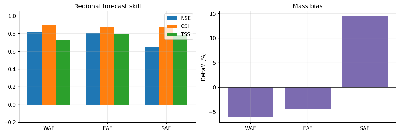
We evaluate continuous depth and event-threshold skill. NSE measures hydrograph agreement, CSI and TSS measure flooded-threshold classification, and delta_mass reports signed volume/depth bias.
[11]:
def predict_arrays(indices):
    out = model(
        tf.convert_to_tensor(X[indices]),
        tf.convert_to_tensor(S[indices]),
        training=False,
    )
    pred = out["depth"].numpy()
    prob = out["exceedance_probability"].numpy()
    features = out["features"].numpy()
    return pred, prob, features


pred_test, prob_test, features_test = predict_arrays(test_idx)
y_test = Y[test_idx]
region_test = regions[test_idx]

rows = []
for spec in REGIONS:
    mask = region_test == spec.code
    yt = y_test[mask].reshape(-1)
    yp = pred_test[mask].reshape(-1)
    rows.append(
        {
            "region": spec.code,
            "NSE": nash_sutcliffe_efficiency(yt, yp),
            "CSI": critical_success_index(yt, yp, threshold=FLOOD_THRESHOLD),
            "TSS": true_skill_statistic(yt, yp, threshold=FLOOD_THRESHOLD),
            "delta_mass_%": delta_mass(yt, yp),
        }
    )

for row in rows:
    print(
        f"{row['region']}: NSE={row['NSE']:.3f} "
        f"CSI={row['CSI']:.3f} TSS={row['TSS']:.3f} "
        f"DeltaM={row['delta_mass_%']:.2f}%"
    )
WAF: NSE=0.819 CSI=0.897 TSS=0.732 DeltaM=-6.12%
EAF: NSE=0.801 CSI=0.877 TSS=0.790 DeltaM=-4.36%
SAF: NSE=0.652 CSI=0.871 TSS=0.782 DeltaM=14.39%
[12]:
def plot_metric_bars(rows):
    labels = [r["region"] for r in rows]
    metrics = ["NSE", "CSI", "TSS"]
    x = np.arange(len(labels))
    width = 0.24
    fig, axes = plt.subplots(1, 2, figsize=(11, 3.8))
    for i, metric in enumerate(metrics):
        axes[0].bar(
            x + (i - 1) * width,
            [r[metric] for r in rows],
            width,
            label=metric,
        )
    axes[0].set_xticks(x, labels)
    axes[0].set_ylim(-0.2, 1.05)
    axes[0].set_title("Regional forecast skill")
    axes[0].legend()

    axes[1].bar(labels, [r["delta_mass_%"] for r in rows], color="#7c6bb0")
    axes[1].axhline(0, color="#222", lw=1)
    axes[1].set_title("Mass bias")
    axes[1].set_ylabel("DeltaM (%)")
    fig.tight_layout()
    return fig

plot_metric_bars(rows)
plt.show()
7. Hydrograph Interpretation
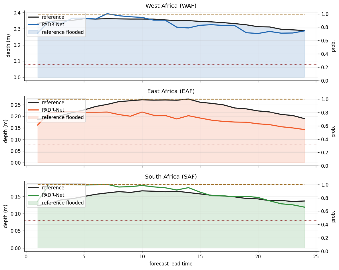
Each panel compares reference flood depth with PADR-Net depth at the same forecast horizon. The shaded region indicates where the reference is above the flood threshold.
[13]:
def plot_region_forecasts(indices, pred, prob):
    fig, axes = plt.subplots(3, 1, figsize=(10, 8), sharex=True)
    test_events = [events[i] for i in indices]
    for ax, spec in zip(axes, REGIONS):
        candidates = [j for j, e in enumerate(test_events) if e["region"] == spec.code]
        # Choose a visible event near the regional 80th percentile.
        peaks = [float(Y[indices[j]].max()) for j in candidates]
        chosen = candidates[int(np.argsort(peaks)[max(0, int(0.8 * len(peaks)) - 1)])]
        ref = Y[indices[chosen], :, 0]
        yh = pred[chosen, :, 0]
        pp = prob[chosen, :, 0]
        t = np.arange(1, HORIZON + 1)
        ax.plot(t, ref, color="#222", lw=2.2, label="reference")
        ax.plot(t, yh, color=spec.color, lw=2.2, label="PADR-Net")
        ax.fill_between(
            t,
            0,
            ref,
            where=ref >= FLOOD_THRESHOLD,
            color=spec.color,
            alpha=0.16,
            label="reference flooded",
        )
        ax2 = ax.twinx()
        ax2.plot(t, pp, color="#9c6b21", lw=1.6, ls="--", label="exceedance")
        ax2.set_ylim(0, 1.05)
        ax2.set_ylabel("prob.")
        ax.axhline(FLOOD_THRESHOLD, color="#8b1e1e", lw=1.0, ls=":")
        ax.set_title(f"{spec.name} ({spec.code})")
        ax.set_ylabel("depth (m)")
        ax.legend(loc="upper left")
    axes[-1].set_xlabel("forecast lead time")
    fig.tight_layout()
    return fig

plot_region_forecasts(test_idx, pred_test, prob_test)
plt.show()
8. Spatial-Style PADR-Net Diagnostic Map
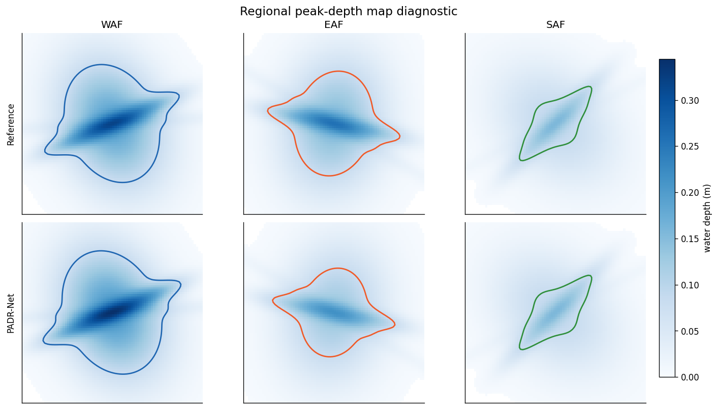
For papers and reports, hydrographs are not always enough. The helper below turns a regional peak depth into a synthetic flood-depth field so we can show the same idea as a 2x3 map:
first row: reference hydrodynamic response;
second row: PADR-Net forecast at the same peak time;
shared colorbar: water depth in metres.
With real data, replace make_spatial_field with your gridded reference and PADR-Net gridded forecast arrays.
[14]:
def make_spatial_field(amplitude, region_index, n=80):
    yy, xx = np.mgrid[-1:1:complex(n), -1:1:complex(n)]
    angle = [0.4, -0.2, 0.8][region_index]
    xr = xx * np.cos(angle) - yy * np.sin(angle)
    yr = xx * np.sin(angle) + yy * np.cos(angle)
    basin = np.exp(-((xr / 0.55) ** 2 + (yr / 0.75) ** 2))
    channel = np.exp(-(yr / 0.11) ** 2) * np.exp(-(xr / 0.9) ** 4)
    tributary = 0.55 * np.exp(-((yr - 0.35 * xr) / 0.09) ** 2)
    field = amplitude * (0.55 * basin + 0.35 * channel + 0.10 * tributary)
    field[field < 0.002] = np.nan
    return field


def plot_spatial_diagnostic(indices, pred):
    fig, axes = plt.subplots(2, 3, figsize=(12, 6.4), constrained_layout=True)
    vmax = 0.0
    fields = []
    for i, spec in enumerate(REGIONS):
        region_pos = np.where(regions[indices] == spec.code)[0]
        peak_order = np.argsort(Y[indices[region_pos]].max(axis=(1, 2)))
        chosen = region_pos[peak_order[int(0.75 * len(peak_order))]]
        ref_peak = float(Y[indices[chosen]].max())
        pred_peak = float(pred[chosen].max())
        ref_field = make_spatial_field(ref_peak, i)
        pred_field = make_spatial_field(pred_peak, i)
        fields.append((ref_field, pred_field, spec))
        vmax = max(vmax, np.nanmax(ref_field), np.nanmax(pred_field))

    for col, (ref_field, pred_field, spec) in enumerate(fields):
        for row, field in enumerate([ref_field, pred_field]):
            ax = axes[row, col]
            im = ax.imshow(field, cmap="Blues", vmin=0, vmax=vmax)
            ax.contour(
                np.nan_to_num(field, nan=0.0),
                levels=[FLOOD_THRESHOLD],
                colors=[spec.color],
                linewidths=1.6,
            )
            ax.set_xticks([])
            ax.set_yticks([])
            if row == 0:
                ax.set_title(f"{spec.code}")
            if col == 0:
                ax.set_ylabel(["Reference", "PADR-Net"][row])
    cbar = fig.colorbar(im, ax=axes.ravel().tolist(), shrink=0.86, pad=0.02)
    cbar.set_label("water depth (m)")
    fig.suptitle("Regional peak-depth map diagnostic", y=1.03, fontsize=14)
    return fig

plot_spatial_diagnostic(test_idx, pred_test)
plt.show()
9. Latent Features and Regional Transfer
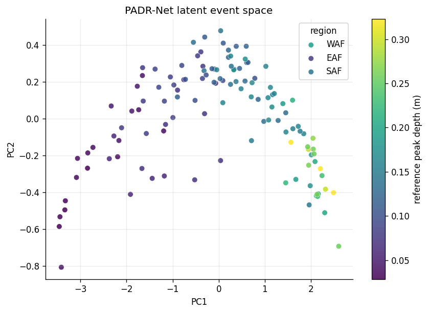
The features output can be used for diagnostics. Here we reduce the latent vectors to two principal directions and color the points by region. A strong model should not merely memorize region identity; it should organize events by hydrological response and severity.
[15]:
def pca2(values):
    centered = values - values.mean(axis=0, keepdims=True)
    _, _, vt = np.linalg.svd(centered, full_matrices=False)
    return centered @ vt[:2].T

coords = pca2(features_test)
peak_depth = y_test.max(axis=(1, 2))

fig, ax = plt.subplots(figsize=(7.2, 5.2))
for spec in REGIONS:
    mask = region_test == spec.code
    sc = ax.scatter(
        coords[mask, 0],
        coords[mask, 1],
        c=peak_depth[mask],
        cmap="viridis",
        s=40,
        alpha=0.85,
        label=spec.code,
        edgecolor="white",
        linewidth=0.4,
    )
ax.set_title("PADR-Net latent event space")
ax.set_xlabel("PC1")
ax.set_ylabel("PC2")
ax.legend(title="region")
cbar = fig.colorbar(sc, ax=ax)
cbar.set_label("reference peak depth (m)")
fig.tight_layout()
plt.show()
10. Optional: PyTorch Backend Smoke Test
The public factory is backend-neutral. The PyTorch implementation uses the same PADRNetConfig and returns the same dictionary keys. This cell is a smoke test; the training loop above remains TensorFlow-specific.
[16]:
try:
    import torch

    torch_model = PADRNet(config, backend="torch")
    torch_out = torch_model(
        torch.zeros(2, LOOKBACK, INPUT_DIM),
        torch.zeros(2, STATIC_DIM),
    )
    print(type(torch_model).__name__)
    for key, value in torch_out.items():
        print(f"{key:24s}", tuple(value.shape))
except Exception as exc:
    print("PyTorch smoke test skipped:", type(exc).__name__, exc)
TorchPADRNet
depth                    (2, 24, 1)
exceedance_probability   (2, 24, 1)
features                 (2, 48)
11. Exercises
Exercise 1: Flood threshold sensitivity
Change FLOOD_THRESHOLD from 0.05 to 0.03 or 0.08, rerun the notebook, and compare CSI, TSS, and the contour line in the spatial map. Which threshold makes false alarms more likely?
Exercise 2: Physics weight ablation
Set lambda_physics=0.0, retrain, and compare the validation loss components and mass bias. Does the model become more accurate in MSE but less physically plausible?
Exercise 3: Leave-one-region-out transfer
Train only on two regions and test on the held-out region. For example, train on WAF+SAF and test on EAF. Which static descriptors help the most when transferring to a new region?
Exercise 4: Replace the synthetic forcing
Replace make_dataset() with real arrays from ERA5/GloFAS/SWE outputs. Keep the same shapes:
X:(batch, lookback, input_dim);S:(batch, static_dim);Y:(batch, forecast_horizon, 1).
The PADR-Net API does not change when the data source changes.
12. Summary
This notebook introduced the complete PADR-Net workflow:
create regional flood-event tensors;
configure
PADRNetConfigwith validated parameters;instantiate
PADRNetwith the TensorFlow backend;train with prediction and physics-aware loss terms;
evaluate NSE, CSI, TSS, and mass bias;
interpret forecasts with hydrographs, spatial maps, and latent event-space diagnostics.
The same structure can now be reused with real hydrodynamic reference outputs or observed flood-depth products.