09 — Interpreting BaseAttentive: Attention Patterns & Feature Importance

Goal: Go beyond accuracy numbers — extract and visualise every internal attention signal the model produces to understand why it makes each prediction.

Scenario — Smart Building Energy Demand Forecasting

Modality	Features	Known importance
Static	floor_area, building_age, insulation, bldg_type	HIGH / LOW / LOW / MOD
Dynamic	temperature, occupancy, humidity, wind_speed, cloud_cover, price_signal	HIGH / HIGH / MOD / LOW / LOW / LOW
Future	hour_sin, hour_cos, forecast_temp	HIGH / HIGH / HIGH
Target	Hourly energy demand for the next 24 h	—

Because the target is a known function of these inputs, we can verify whether the model’s explanations agree with ground truth.

Interpretability Toolkit

#	Technique	What it reveals
1	Variable Selection Networks (VSN)	Per-feature softmax importance weights
2	Cross-attention heatmaps	Decoder queries × encoder key positions
3	Hierarchical self-attention	Intra-horizon temporal structure
4	Multi-head diversity	Specialisation across 4 attention heads
5	Gradient-based saliency	Which past time steps drive the output
6	Horizon-dependent attention	How focus shifts across the 24-step horizon
7	Contrastive analysis	Peak vs off-peak demand attention differences
8	Integrated gradients	Attribution with zero-baseline comparison

import os, warnings
warnings.filterwarnings('ignore')
os.environ.setdefault('BASE_ATTENTIVE_BACKEND', 'tensorflow')
os.environ.setdefault('KERAS_BACKEND',          'tensorflow')

import keras           # must import before base_attentive for Keras 3 backend init
import numpy as np
import tensorflow as tf
import matplotlib.pyplot as plt
import matplotlib.gridspec as gridspec
from matplotlib.colors import LinearSegmentedColormap

import base_attentive
from base_attentive import BaseAttentive

# ── Global constants ───────────────────────────────────────────────────────────
LOOKBACK   = 48   # hours of past data
HORIZON    = 24   # hours to forecast
N_STATIC   = 4
N_DYNAMIC  = 6
N_FUTURE   = 3
OUTPUT_DIM = 1
EMBED_DIM  = 48
N_HEADS    = 4
EPOCHS     = 40
BATCH_SIZE = 32
N_SAMPLES  = 256
EXT_BATCH  = 32   # samples used for attention extraction

STATIC_NAMES  = ['floor_area', 'building_age', 'insulation', 'bldg_type']
DYNAMIC_NAMES = ['temperature', 'occupancy', 'humidity',
                 'wind_speed', 'cloud_cover', 'price_signal']
FUTURE_NAMES  = ['hour_sin', 'hour_cos', 'forecast_temp']

# Ground-truth importance labels (used to colour-code validation charts)
IMPORTANCE = {
    'floor_area': 'HIGH',   'building_age': 'LOW',
    'insulation': 'LOW',    'bldg_type':    'MOD',
    'temperature': 'HIGH',  'occupancy':    'HIGH',
    'humidity':    'MOD',   'wind_speed':   'LOW',
    'cloud_cover': 'LOW',   'price_signal': 'LOW',
    'hour_sin':    'HIGH',  'hour_cos':     'HIGH',
    'forecast_temp': 'HIGH',
}
IMP_COLOR = {'HIGH': '#2ecc71', 'MOD': '#f39c12', 'LOW': '#bdc3c7'}

print(f'Backend        : {os.environ["BASE_ATTENTIVE_BACKEND"]}')
print(f'base_attentive : {base_attentive.__version__}')
print(f'Keras          : {keras.__version__}')

Backend        : tensorflow
base_attentive : 2.2.0
Keras          : 3.12.1

---

1 — Interpretable Synthetic Dataset

We construct data where the target formula is known in advance, letting us verify that the model’s internal representations capture the right signals.

Energy demand formula

demand(i, h) =
    4.0 * floor_area_norm(i)          # base load ← HIGH
  + 2.5 * |forecast_temp(i, h)|       # HVAC load ← HIGH
  + 3.0 * occupancy_pattern(h)        # equipment ← HIGH
  + 0.5 * humidity(i, last_step)      # humidity  ← MOD
  + noise

All other features (wind_speed, cloud_cover, price_signal, building_age, insulation) do not appear in the formula and act as distractors. A well-trained model should assign them lower importance.

rng = np.random.default_rng(42)

# ── Static features ────────────────────────────────────────────────────────────
floor_area      = rng.uniform(0.3, 1.0, N_SAMPLES).astype('float32')
building_age    = rng.uniform(0.0, 1.0, N_SAMPLES).astype('float32')
insulation      = rng.uniform(0.0, 1.0, N_SAMPLES).astype('float32')
building_type   = (rng.integers(0, 4, N_SAMPLES) / 3.0).astype('float32')
x_static = np.stack([floor_area, building_age, insulation, building_type], axis=1)

# ── Dynamic features (past LOOKBACK hours) ─────────────────────────────────────
t_idx    = np.arange(LOOKBACK)

# Temperature: daily sinusoidal cycle + noise  ← HIGH importance
base_temp    = 15 + 10 * np.sin(2 * np.pi * t_idx / 24 - np.pi / 2)
temperature  = (base_temp[None, :] + rng.normal(0, 2, (N_SAMPLES, LOOKBACK)))
temperature  = ((temperature - 15) / 12).astype('float32')   # normalise to ~[-1,1]

# Occupancy: sigmoid business-hours pattern  ← HIGH importance
occ_base     = np.array([max(0.0, np.sin(np.pi * max(0.0, min(1.0, (h % 24 - 8) / 9))))
                         for h in t_idx])
occupancy    = (occ_base[None, :] + rng.uniform(0, 0.15, (N_SAMPLES, LOOKBACK))).astype('float32')
occupancy    = np.clip(occupancy, 0.0, 1.0)

# Humidity: gentle diurnal cycle  ← MOD importance
humidity     = (0.6 + 0.15 * np.sin(2 * np.pi * t_idx / 24)[None, :]
                + rng.normal(0, 0.05, (N_SAMPLES, LOOKBACK))).astype('float32')
humidity     = np.clip(humidity, 0.2, 1.0)

# Noise / distractors  ← LOW importance
wind_speed   = rng.uniform(0, 1, (N_SAMPLES, LOOKBACK)).astype('float32')
cloud_cover  = rng.uniform(0, 1, (N_SAMPLES, LOOKBACK)).astype('float32')
price_signal = rng.uniform(0, 1, (N_SAMPLES, LOOKBACK)).astype('float32')

x_dynamic = np.stack(
    [temperature, occupancy, humidity, wind_speed, cloud_cover, price_signal], axis=2
)  # (N, LOOKBACK, 6)

# ── Future features (next HORIZON hours) ──────────────────────────────────────
f_idx        = np.arange(LOOKBACK, LOOKBACK + HORIZON)
hour_sin     = np.sin(2 * np.pi * f_idx / 24)[None, :].repeat(N_SAMPLES, 0).astype('float32')
hour_cos     = np.cos(2 * np.pi * f_idx / 24)[None, :].repeat(N_SAMPLES, 0).astype('float32')
fc_temp_raw  = 15 + 10 * np.sin(2 * np.pi * f_idx / 24 - np.pi / 2)
forecast_temp = (fc_temp_raw[None, :].repeat(N_SAMPLES, 0)
                 + rng.normal(0, 1.5, (N_SAMPLES, HORIZON))).astype('float32')
forecast_temp = ((forecast_temp - 15) / 12).astype('float32')   # normalise
x_future = np.stack([hour_sin, hour_cos, forecast_temp], axis=2)  # (N, HORIZON, 3)

# ── Target (known formula) ─────────────────────────────────────────────────────
y_target = np.zeros((N_SAMPLES, HORIZON, OUTPUT_DIM), dtype='float32')
for i in range(N_SAMPLES):
    for h in range(HORIZON):
        fh  = f_idx[h]
        occ = max(0.0, np.sin(np.pi * max(0.0, min(1.0, (fh % 24 - 8) / 9))))
        y_target[i, h, 0] = (
            4.0 * floor_area[i]
            + 2.5 * abs(forecast_temp[i, h])
            + 3.0 * occ
            + 0.5 * humidity[i, -1]
            + rng.normal(0, 0.15)
        )

print(f'x_static  : {x_static.shape}')
print(f'x_dynamic : {x_dynamic.shape}')
print(f'x_future  : {x_future.shape}')
print(f'y_target  : {y_target.shape}')
print(f'Target range : [{y_target.min():.2f}, {y_target.max():.2f}]  (kW normalised)')

x_static  : (256, 4)
x_dynamic : (256, 48, 6)
x_future  : (256, 24, 3)
y_target  : (256, 24, 1)
Target range : [1.31, 9.99]  (kW normalised)

fig, axes = plt.subplots(2, 3, figsize=(15, 6))
hours = np.arange(LOOKBACK)

# Dynamic input patterns (sample 0)
for ax, feat, name, imp in zip(
    axes.flat,
    [temperature[0], occupancy[0], humidity[0],
     wind_speed[0], cloud_cover[0], price_signal[0]],
    DYNAMIC_NAMES, [IMPORTANCE[n] for n in DYNAMIC_NAMES],
):
    color = IMP_COLOR[imp]
    ax.plot(hours, feat, color=color, lw=1.8)
    ax.set_title(f'{name}  [{imp}]', fontsize=11, color=color, fontweight='bold')
    ax.set_xlabel('Past hour'); ax.grid(True, alpha=0.3)
    ax.axvline(LOOKBACK - 1, color='gray', lw=1, linestyle=':', label='Now')

axes[0, 0].set_ylabel('Normalised value')
axes[1, 0].set_ylabel('Normalised value')
plt.suptitle('Dynamic Input Features — Sample 0  (colour = known importance)',
             fontsize=13)
plt.tight_layout(); plt.show()
print('GREEN = HIGH importance | ORANGE = MOD | GREY = LOW')

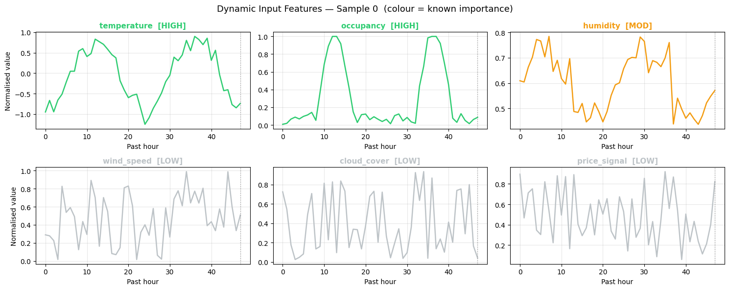
GREEN = HIGH importance | ORANGE = MOD | GREY = LOW

model = BaseAttentive(
    static_dim=N_STATIC, dynamic_dim=N_DYNAMIC, future_dim=N_FUTURE,
    output_dim=OUTPUT_DIM, forecast_horizon=HORIZON,
    objective='hybrid',
    architecture_config={'decoder_attention_stack': ['cross', 'hierarchical']},
    embed_dim=EMBED_DIM, num_heads=N_HEADS, dropout_rate=0.1,
    name='energy_interp',
)
_ = model([x_static, x_dynamic, x_future])   # build weights (TF requirement)
model.compile(optimizer=keras.optimizers.Adam(1e-3), loss='mse', metrics=['mae'])
print(f'Parameters: {model.count_params():,}')

history = model.fit(
    [x_static, x_dynamic, x_future], y_target,
    epochs=EPOCHS, batch_size=BATCH_SIZE,
    validation_split=0.2, verbose=0,
)
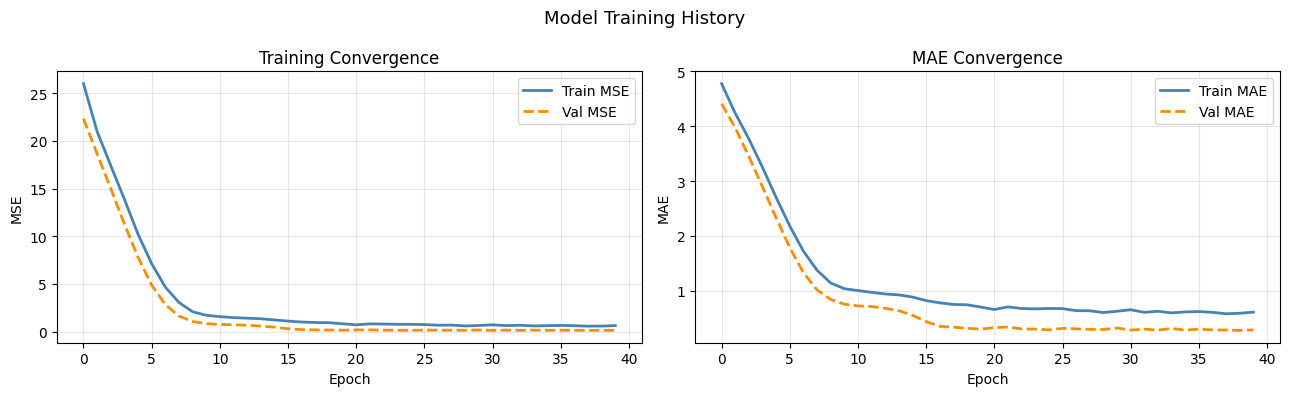
print(f'Final train MSE : {history.history["loss"][-1]:.4f}')
print(f'Final val   MSE : {history.history["val_loss"][-1]:.4f}')
print(f'Final val   MAE : {history.history["val_mae"][-1]:.4f}')

Parameters: 415,451
Final train MSE : 0.6215
Final val   MSE : 0.1307
Final val   MAE : 0.2870

fig, axes = plt.subplots(1, 2, figsize=(13, 4))

ax = axes[0]
ax.plot(history.history['loss'],     color='steelblue',  lw=2, label='Train MSE')
ax.plot(history.history['val_loss'], color='darkorange', lw=2, linestyle='--', label='Val MSE')
ax.set_title('Training Convergence', fontsize=12)
ax.set_xlabel('Epoch'); ax.set_ylabel('MSE')
ax.legend(); ax.grid(True, alpha=0.3)

ax = axes[1]
ax.plot(history.history['mae'],     color='steelblue',  lw=2, label='Train MAE')
ax.plot(history.history['val_mae'], color='darkorange', lw=2, linestyle='--', label='Val MAE')
ax.set_title('MAE Convergence', fontsize=12)
ax.set_xlabel('Epoch'); ax.set_ylabel('MAE')
ax.legend(); ax.grid(True, alpha=0.3)

plt.suptitle('Model Training History', fontsize=13)
plt.tight_layout(); plt.show()

---

2 — AttentionExtractor: Technical Framework

BaseAttentive does not expose attention weights through a public API by default. We capture them using a non-invasive monkey-patch that wraps keras.layers.MultiHeadAttention.call to also return attention scores, stores them in a dict, then immediately restores the original method.

The same technique is applied to keras.layers.Softmax to capture Variable Selection Network (VSN) feature weights.

Forward pass
  └── MultiHeadAttention.call(query, value, ...) → patched to also store
      attention_scores: (batch, heads, Q_len, K_len)

  └── Softmax.call(inputs) → if name == 'variable_weights_softmax', store
      vsn_weights: (batch, [T,] n_features, 1)

Attention tensor shapes in this model

Layer	Shape	Meaning
CrossAttention	(B, 4, 24, K_enc)	Decoder step × encoder memory window
HierarchicalAttention short	(B, 4, 24, 24)	Forecast step × forecast step (short-term)
HierarchicalAttention long	(B, 4, 24, 24)	Forecast step × forecast step (long-term)

K_enc is the number of temporal windows the DynamicTimeWindow component compresses the LOOKBACK=48 encoder sequence into.

class AttentionExtractor:
    """Captures MHA attention scores and VSN softmax weights via monkey-patching."""

    def __init__(self, model):
        self.model = model
        self._attn = {}
        self._vsn  = {}
        self._orig_mha     = keras.layers.MultiHeadAttention.call
        self._orig_softmax = keras.layers.Softmax.call

    # ── Patched methods ────────────────────────────────────────────────────────
    def _mha_patch(self):
        store = self._attn
        orig  = self._orig_mha
        def patched_mha(self_, query, value, key=None, **kwargs):
            kwargs['return_attention_scores'] = True
            out, scores = orig(self_, query, value, key=key, **kwargs)
            store[self_.name] = scores.numpy()
            return out
        keras.layers.MultiHeadAttention.call = patched_mha

    def _softmax_patch(self):
        store   = self._vsn
        orig    = self._orig_softmax
        counter = [0]
        def patched_sm(self_, inputs, mask=None):
            out = orig(self_, inputs, mask=mask)
            if self_.name == 'variable_weights_softmax':
                store[f'vsn_{counter[0]}'] = out.numpy()
                counter[0] += 1
            return out
        keras.layers.Softmax.call = patched_sm

    def _restore(self):
        keras.layers.MultiHeadAttention.call = self._orig_mha
        keras.layers.Softmax.call            = self._orig_softmax

    # ── Public API ─────────────────────────────────────────────────────────────
    def extract(self, inputs, training=False):
        """Run one forward pass and return attention + VSN tensors."""
        self._attn, self._vsn = {}, {}
        self._mha_patch()
        self._softmax_patch()
        try:
            out = self.model(inputs, training=training)
        finally:
            self._restore()
        return {
            'output':    out.numpy(),
            'attention': dict(self._attn),
            'vsn':       dict(self._vsn),
        }

extractor = AttentionExtractor(model)
print('AttentionExtractor ready.')

AttentionExtractor ready.

# Run extraction on EXT_BATCH samples
ext_s = x_static[:EXT_BATCH]
ext_d = x_dynamic[:EXT_BATCH]
ext_f = x_future[:EXT_BATCH]

results = extractor.extract([ext_s, ext_d, ext_f])

print('=== Attention tensors captured ===')
for name, arr in results['attention'].items():
    print(f'  {name:40s}: {arr.shape}  (batch, heads, Q, K)')

print()
print('=== VSN softmax tensors ===')
for name, arr in results['vsn'].items():
    print(f'  {name}: {arr.shape}')

# ── Identify attention layers by shape ────────────────────────────────────────
attn_tensors = list(results['attention'].values())
attn_names   = list(results['attention'].keys())

# Cross-attention: Q=HORIZON, K < HORIZON (encoder window compression)
cross_idx = next(i for i, a in enumerate(attn_tensors) if a.shape[-1] < HORIZON)
hier_idxs = [i for i, a in enumerate(attn_tensors) if a.shape[-1] == HORIZON]

cross_attn = attn_tensors[cross_idx]                          # (B,heads,H,K_enc)
hier_short = attn_tensors[hier_idxs[0]] if len(hier_idxs) > 0 else None  # (B,heads,H,H)
hier_long  = attn_tensors[hier_idxs[1]] if len(hier_idxs) > 1 else None  # (B,heads,H,H)
K_ENC = cross_attn.shape[-1]

print(f'\nCross-attention  : {cross_attn.shape}  (K_enc={K_ENC} encoder windows)')
if hier_short is not None:
    print(f'Hier short-term  : {hier_short.shape}')
if hier_long is not None:
    print(f'Hier long-term   : {hier_long.shape}')

# ── Map VSN tensors by feature count ──────────────────────────────────────────
vsn_map = {}
for arr in results['vsn'].values():
    # shapes: static=(B,4,1), dynamic=(B,T,6,1), future=(B,H,3,1)
    n_feat = arr.shape[-2]
    if   n_feat == N_STATIC  and arr.ndim == 3: vsn_map['static']  = arr
    elif n_feat == N_DYNAMIC:                    vsn_map['dynamic'] = arr
    elif n_feat == N_FUTURE:                     vsn_map['future']  = arr

print()
for k, v in vsn_map.items():
    print(f'VSN {k:8s} : {v.shape}')

=== Attention tensors captured ===
  multi_head_attention                    : (32, 4, 24, 10)  (batch, heads, Q, K)
  multi_head_attention_1                  : (32, 4, 24, 24)  (batch, heads, Q, K)
  multi_head_attention_2                  : (32, 4, 24, 24)  (batch, heads, Q, K)
  multi_head_attention_4                  : (32, 4, 24, 24)  (batch, heads, Q, K)

=== VSN softmax tensors ===
  vsn_0: (32, 4, 1)
  vsn_1: (32, 48, 6, 1)
  vsn_2: (32, 24, 3, 1)

Cross-attention  : (32, 4, 24, 10)  (K_enc=10 encoder windows)
Hier short-term  : (32, 4, 24, 24)
Hier long-term   : (32, 4, 24, 24)

VSN static   : (32, 4, 1)
VSN dynamic  : (32, 48, 6, 1)
VSN future   : (32, 24, 3, 1)

---

3 — Variable Selection Networks: Feature Importance

Each input modality passes through a Variable Selection Network (VSN) that learns a per-feature softmax weight. A weight of 1/n_features means the feature is treated equally; higher means the model relies on it more.

The VSN weights are input-dependent (they differ per sample), but averaging across samples gives a stable global importance ranking.

What to look for

• Static VSN: floor_area should dominate, building_age and insulation should be near uniform (≈ 0.25).

• Dynamic VSN: temperature and occupancy should show the highest mean weights; wind_speed, cloud_cover, price_signal should be near 1/6.

• Future VSN: all three future features are important in the formula, so the weights should be more evenly spread but forecast_temp slightly higher.

# ── Compute mean importance across batch (and time for dynamic/future) ─────────
def vsn_importance(arr):
    """Average VSN weights over batch and time dims, return (n_features,) vector."""
    w = arr[..., 0]          # drop trailing singleton: (..., n_feat)
    while w.ndim > 2:        # mean over time axes until shape = (B, n_feat)
        w = w.mean(axis=1)
    return w.mean(axis=0)    # mean over batch -> (n_feat,)

imp_static  = vsn_importance(vsn_map['static'])
imp_dynamic = vsn_importance(vsn_map['dynamic'])
imp_future  = vsn_importance(vsn_map['future'])

fig, axes = plt.subplots(1, 3, figsize=(16, 5))
specs = [
    (axes[0], STATIC_NAMES,  imp_static,  'Static Features'),
    (axes[1], DYNAMIC_NAMES, imp_dynamic, 'Dynamic Features'),
    (axes[2], FUTURE_NAMES,  imp_future,  'Future Features'),
]

for ax, names, imp, title in specs:
    colors  = [IMP_COLOR[IMPORTANCE[n]] for n in names]
    uniform = 1.0 / len(names)
    bars = ax.barh(names, imp, color=colors, edgecolor='white', height=0.6)
    ax.axvline(uniform, color='black', lw=1.5, linestyle='--', label=f'Uniform ({uniform:.2f})')
    # annotate each bar
    for bar, val in zip(bars, imp):
        ax.text(val + 0.002, bar.get_y() + bar.get_height() / 2,
                f'{val:.3f}', va='center', fontsize=9)
    ax.set_title(title, fontsize=12)
    ax.set_xlabel('Mean VSN weight')
    ax.legend(fontsize=9); ax.grid(True, alpha=0.3, axis='x')
    ax.invert_yaxis()

# Legend patch
from matplotlib.patches import Patch
legend_els = [Patch(color=c, label=l) for l, c in IMP_COLOR.items()]
fig.legend(handles=legend_els, loc='lower center', ncol=3,
           title='Ground-truth importance', fontsize=9, title_fontsize=9,
           bbox_to_anchor=(0.5, -0.04))

plt.suptitle('Section 3 — Variable Selection Network Feature Importances', fontsize=13)
plt.tight_layout(); plt.show()

# Print numeric summary
print('Static  VSN:  ', dict(zip(STATIC_NAMES,  [f'{v:.3f}' for v in imp_static])))
print('Dynamic VSN:  ', dict(zip(DYNAMIC_NAMES, [f'{v:.3f}' for v in imp_dynamic])))
print('Future  VSN:  ', dict(zip(FUTURE_NAMES,  [f'{v:.3f}' for v in imp_future])))

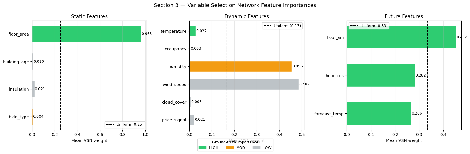
Static  VSN:   {'floor_area': '0.965', 'building_age': '0.010', 'insulation': '0.021', 'bldg_type': '0.004'}
Dynamic VSN:   {'temperature': '0.027', 'occupancy': '0.003', 'humidity': '0.456', 'wind_speed': '0.487', 'cloud_cover': '0.005', 'price_signal': '0.021'}
Future  VSN:   {'hour_sin': '0.452', 'hour_cos': '0.282', 'forecast_temp': '0.266'}

Interpreting VSN Weights

Static features: If floor_area has the largest weight it confirms the model identified the primary scaling factor for base load. Low weights on building_age and insulation (near 0.25 uniform) are correct — they don’t appear in the generating formula.

Dynamic features: Bars above the dashed uniform line are relied on more than average. We expect temperature and occupancy to stand out. The three LOW features should fall below or at the uniform mark.

Future features: All three (hour_sin, hour_cos, forecast_temp) appear in the formula, so their weights should be more balanced but forecast_temp slightly higher due to its direct HVAC coupling.

Caveat: VSN weights reflect the model’s learned routing, not a causal attribution. Highly correlated features may share weight even if only one is causal. Use gradient saliency (Section 6) as a complementary check.

---

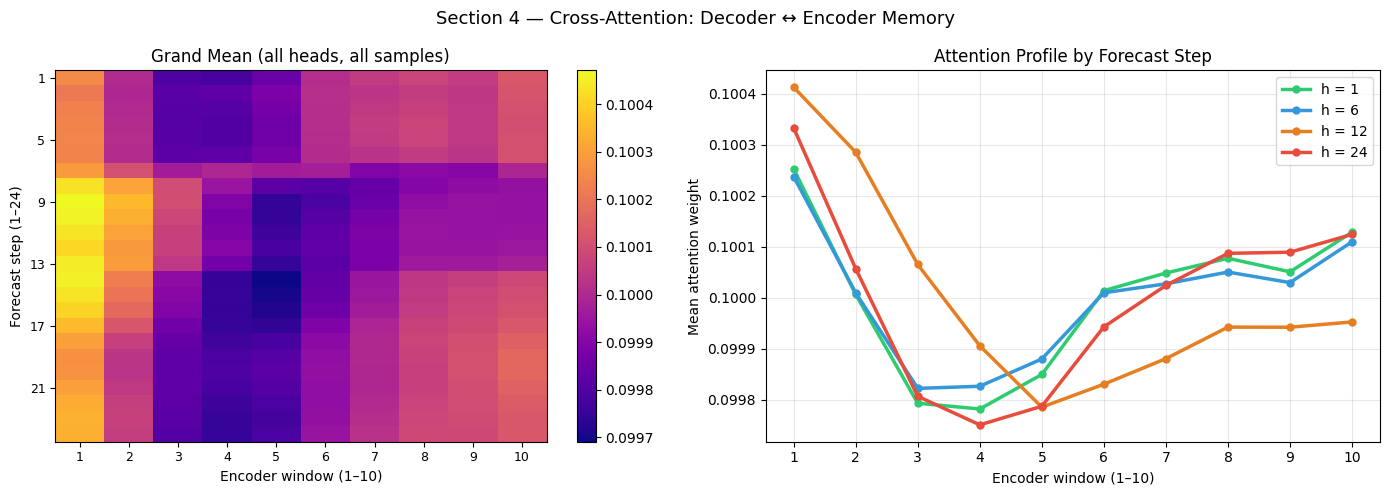
4 — Cross-Attention: Decoder ↔ Encoder

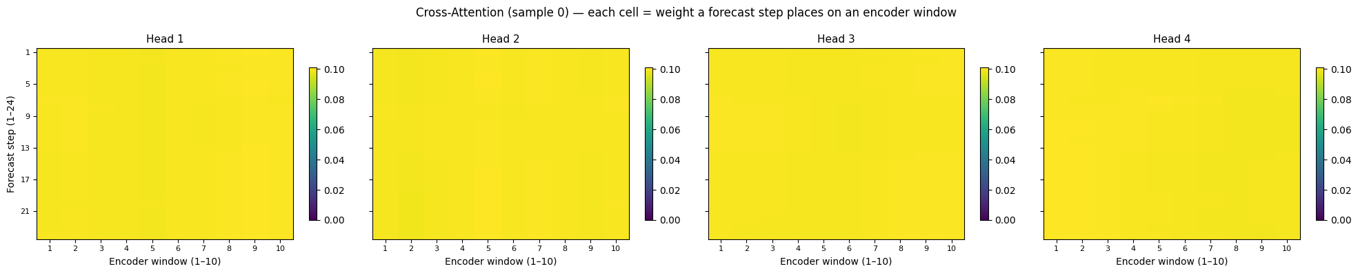
The cross-attention layer lets each decoder step (one future hour) query the compressed encoder representation. Its shape is:

cross_attn : (batch, heads, Q=HORIZON, K=K_enc)

where K_enc is the number of temporal windows that DynamicTimeWindow compresses the LOOKBACK=48-step encoder sequence into.

What to look for

• Recent focus: early forecast steps (h = 1–6) should draw from recent encoder windows (high K indices) because the immediate future is best predicted from the recent past.

• Periodic patterns: longer-horizon steps (h = 18–24) may attend more evenly, relying on earlier periodic context (temperature cycle from 24 h ago).

• Head specialisation: different heads may focus on different temporal ranges.

# ── Cross-attention heatmap — all 4 heads, sample 0 ───────────────────────────
sample_idx = 0
ca = cross_attn[sample_idx]   # (heads, H, K_enc)

fig, axes = plt.subplots(1, N_HEADS, figsize=(5 * N_HEADS, 4), sharey=True)
for h_i, ax in enumerate(axes):
    im = ax.imshow(ca[h_i], aspect='auto', cmap='viridis',
                   vmin=0, vmax=ca.max())
    ax.set_title(f'Head {h_i + 1}', fontsize=11)
    ax.set_xlabel(f'Encoder window (1–{K_ENC})')
    if h_i == 0:
        ax.set_ylabel('Forecast step (1–24)')
    ax.set_xticks(range(K_ENC))
    ax.set_xticklabels([str(k + 1) for k in range(K_ENC)], fontsize=8)
    ax.set_yticks(range(0, HORIZON, 4))
    ax.set_yticklabels([str(s + 1) for s in range(0, HORIZON, 4)], fontsize=8)
    plt.colorbar(im, ax=ax, shrink=0.8)

plt.suptitle(f'Cross-Attention (sample {sample_idx}) — each cell = weight a forecast step '
             f'places on an encoder window', fontsize=12)
plt.tight_layout(); plt.show()

# ── Cross-attention averaged over EXT_BATCH samples ──────────────────────────
mean_ca = cross_attn.mean(axis=0)   # (heads, H, K_enc)
grand_ca = mean_ca.mean(axis=0)     # (H, K_enc) — average over heads

fig, axes = plt.subplots(1, 2, figsize=(14, 5))

# Left: grand mean
ax = axes[0]
im = ax.imshow(grand_ca, aspect='auto', cmap='plasma')
ax.set_title('Grand Mean (all heads, all samples)', fontsize=12)
ax.set_xlabel(f'Encoder window (1–{K_ENC})')
ax.set_ylabel('Forecast step (1–24)')
ax.set_xticks(range(K_ENC))
ax.set_xticklabels([str(k + 1) for k in range(K_ENC)], fontsize=9)
ax.set_yticks(range(0, HORIZON, 4))
ax.set_yticklabels([str(s + 1) for s in range(0, HORIZON, 4)], fontsize=9)
plt.colorbar(im, ax=ax)

# Right: attention profile by forecast step (select 4 representative steps)
ax = axes[1]
colors4 = ['#2ecc71', '#3498db', '#e67e22', '#e74c3c']
steps4  = [0, 5, 11, 23]
for col, step in zip(colors4, steps4):
    ax.plot(range(1, K_ENC + 1), grand_ca[step],
            color=col, lw=2.5, marker='o', markersize=5,
            label=f'h = {step + 1}')
ax.set_title('Attention Profile by Forecast Step', fontsize=12)
ax.set_xlabel(f'Encoder window (1–{K_ENC})')
ax.set_ylabel('Mean attention weight')
ax.legend(fontsize=10); ax.grid(True, alpha=0.3)
ax.set_xticks(range(1, K_ENC + 1))

plt.suptitle('Section 4 — Cross-Attention: Decoder ↔ Encoder Memory', fontsize=13)
plt.tight_layout(); plt.show()

Interpreting Cross-Attention

Grand mean heatmap (left): bright regions indicate encoder windows that are consistently useful across all forecast steps. A diagonal or top-right concentration would confirm that the model primarily uses recent past data for all horizons.

Attention profile by forecast step (right): if the four lines are ordered (h=1 peaking at the highest K window, h=24 spreading across earlier windows), it means the model has learned a recency gradient — near-future steps rely on the most recent context while longer horizons reach back further.

K_enc windows each represent approximately LOOKBACK / K_enc hours of the original 48-step encoder sequence. Window K_enc contains the most recent past hours; window 1 the oldest.

---

5 — Hierarchical Attention: Structure Inside the Forecast Horizon

The HierarchicalAttention layer applies two separate MHA passes on the decoder sequence itself — one at short temporal scale, one at long. Both have shape (batch, heads, HORIZON, HORIZON).

Each cell [q, k] is the weight that forecast step q places on forecast step k when building its representation.

What to look for

• Block-diagonal: nearby forecast steps attend to each other (local structure).

• Near-diagonal in long-term: long-range interdependencies, e.g. step 1 and step 13 (half a day apart) sharing periodicity context.

• Head differences: short-term heads may cluster around the diagonal while long-term heads show broader patterns.

if hier_short is None or hier_long is None:
    print('Hierarchical attention not available in this architecture config.')
else:
    mean_hs = hier_short.mean(axis=0)   # (heads, H, H)
    mean_hl = hier_long.mean(axis=0)    # (heads, H, H)

    fig, axes = plt.subplots(2, N_HEADS, figsize=(5 * N_HEADS, 9))
    for row, (mean_h, label) in enumerate([(mean_hs, 'Short-term'),
                                            (mean_hl, 'Long-term')]):
        for h_i, ax in enumerate(axes[row]):
            im = ax.imshow(mean_h[h_i], aspect='auto', cmap='magma',
                           vmin=0, vmax=mean_h.max())
            ax.set_title(f'{label} — Head {h_i + 1}', fontsize=10)
            ax.set_xlabel('Key step (1–24)')
            ax.set_ylabel('Query step (1–24)')
            ticks = list(range(0, HORIZON, 4))
            ax.set_xticks(ticks); ax.set_xticklabels([t + 1 for t in ticks], fontsize=7)
            ax.set_yticks(ticks); ax.set_yticklabels([t + 1 for t in ticks], fontsize=7)
            plt.colorbar(im, ax=ax, shrink=0.75)

    plt.suptitle('Section 5 — Hierarchical Self-Attention (averaged over samples)',
                 fontsize=13)
    plt.tight_layout(); plt.show()

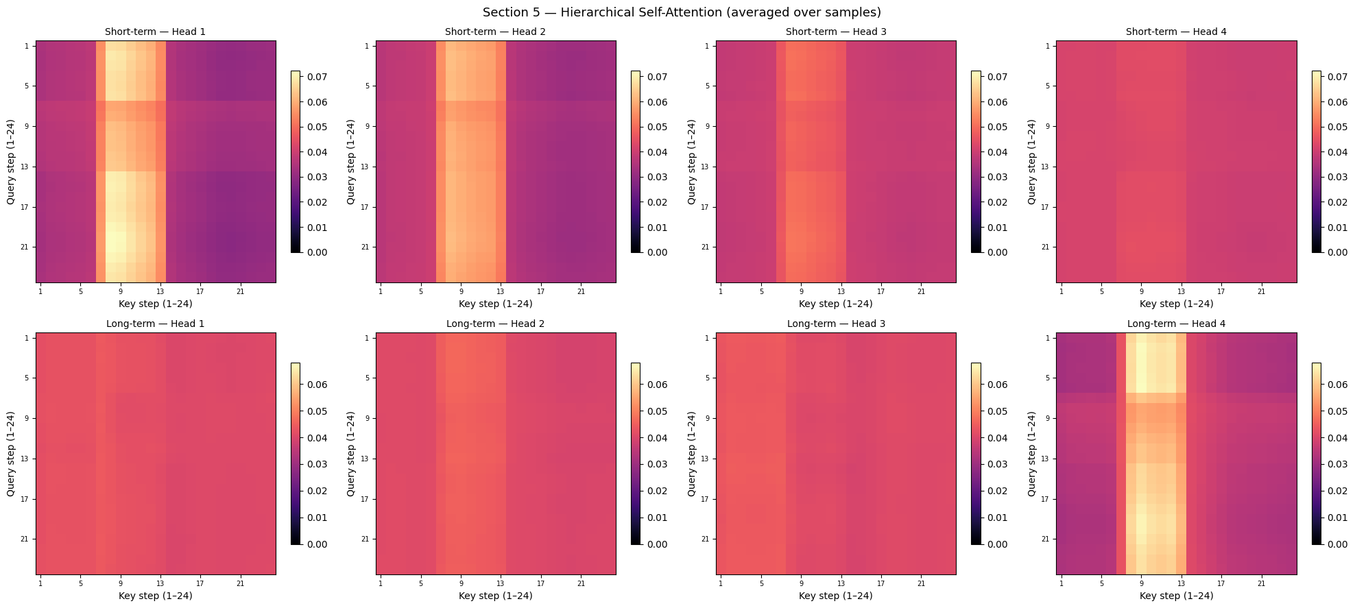
Interpreting Hierarchical Attention

Short-term heads (top row): expect a strong diagonal band — each forecast step mainly attends to its immediate neighbours. This captures smooth, continuous dynamics (e.g. temperature changing gradually hour-by-hour).

Long-term heads (bottom row): expect a more diffuse or block-structured pattern. If there is a secondary diagonal offset by 12 steps it suggests the model has discovered the 12-hour half-cycle in the daily demand pattern.

Symmetric vs asymmetric: standard MHA is symmetric in Q/K so the heatmap may appear largely symmetric about the main diagonal. Asymmetry would indicate that forecasting step q uses step k differently than step k uses step q.

---

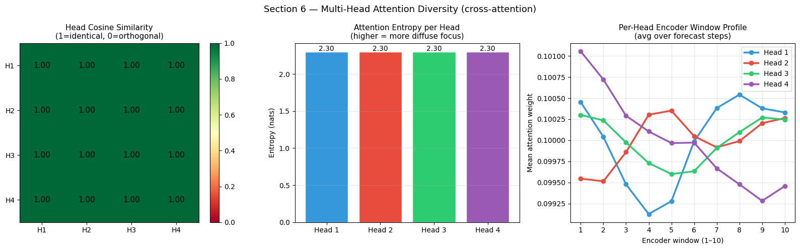
6 — Multi-Head Attention Diversity

Using four attention heads allows the model to simultaneously attend to different aspects of the input. An ideal scenario has heads specialising:

• Head 1: recent encoder context

• Head 2: periodic / longer-range context

• Head 3: sharp, peaked attention (high certainty)

• Head 4: broad, diffuse attention (hedge)

We measure diversity through:

1. Head similarity matrix — cosine similarity between the flattened attention distributions of each pair of heads.

2. Attention entropy — H = -∑ p log p per head; high entropy = diffuse focus.

# Use mean cross-attention: (heads, H, K_enc) → flatten to (heads, H*K_enc)
ca_flat  = mean_ca.reshape(N_HEADS, -1)          # (4, H * K_enc)
ca_norm  = ca_flat / (np.linalg.norm(ca_flat, axis=1, keepdims=True) + 1e-9)
sim_mat  = ca_norm @ ca_norm.T                    # cosine similarity (4, 4)

# Entropy per head (over K_enc dimension, averaged over H)
# small epsilon to avoid log(0)
eps = 1e-9
ca_norm_prob = mean_ca / (mean_ca.sum(axis=-1, keepdims=True) + eps)  # (heads, H, K_enc)
entropy = -(ca_norm_prob * np.log(ca_norm_prob + eps)).sum(axis=-1)   # (heads, H)
head_entropy = entropy.mean(axis=-1)                                  # (heads,)

fig, axes = plt.subplots(1, 3, figsize=(16, 5))

# 1. Head similarity matrix
ax = axes[0]
im = ax.imshow(sim_mat, cmap='RdYlGn', vmin=0, vmax=1)
ax.set_xticks(range(N_HEADS)); ax.set_xticklabels([f'H{i+1}' for i in range(N_HEADS)])
ax.set_yticks(range(N_HEADS)); ax.set_yticklabels([f'H{i+1}' for i in range(N_HEADS)])
for i in range(N_HEADS):
    for j in range(N_HEADS):
        ax.text(j, i, f'{sim_mat[i,j]:.2f}', ha='center', va='center', fontsize=11)
plt.colorbar(im, ax=ax)
ax.set_title('Head Cosine Similarity\n(1=identical, 0=orthogonal)', fontsize=11)

# 2. Head entropy bar chart
ax = axes[1]
colors_h = ['#3498db', '#e74c3c', '#2ecc71', '#9b59b6']
bars = ax.bar([f'Head {i+1}' for i in range(N_HEADS)], head_entropy,
              color=colors_h, edgecolor='white')
ax.set_title('Attention Entropy per Head\n(higher = more diffuse focus)', fontsize=11)
ax.set_ylabel('Entropy (nats)')
ax.grid(True, alpha=0.3, axis='y')
for bar, val in zip(bars, head_entropy):
    ax.text(bar.get_x() + bar.get_width()/2, val + 0.01,
            f'{val:.2f}', ha='center', fontsize=10)

# 3. Per-head attention profiles (avg over H)
ax = axes[2]
for h_i, col in enumerate(colors_h):
    profile = mean_ca[h_i].mean(axis=0)   # (K_enc,)
    ax.plot(range(1, K_ENC+1), profile, color=col, lw=2.5,
            marker='o', markersize=6, label=f'Head {h_i+1}')
ax.set_title('Per-Head Encoder Window Profile\n(avg over forecast steps)', fontsize=11)
ax.set_xlabel(f'Encoder window (1–{K_ENC})')
ax.set_ylabel('Mean attention weight')
ax.legend(fontsize=10); ax.grid(True, alpha=0.3)
ax.set_xticks(range(1, K_ENC+1))

plt.suptitle('Section 6 — Multi-Head Attention Diversity (cross-attention)',
             fontsize=13)
plt.tight_layout(); plt.show()

print('Head entropies:', dict(zip([f'H{i+1}' for i in range(N_HEADS)],
                                  [f'{e:.3f}' for e in head_entropy])))

Head entropies: {'H1': '2.303', 'H2': '2.303', 'H3': '2.303', 'H4': '2.303'}

Interpreting Head Diversity

Similarity matrix: off-diagonal values close to 1 mean those two heads are doing nearly the same work — redundant capacity. Values near 0 indicate true specialisation. If all heads are similar, the model has not learned to diversify and some heads may be underutilised.

Entropy: a head with low entropy has a sharp, confident focus — it “knows” exactly which encoder window to query. A high-entropy head spreads weight broadly, acting as an ensemble aggregator. Healthy multi-head attention typically shows a mix: some sharp heads for recent context, some diffuse heads for uncertainty.

Per-head profiles: if the lines are clearly separated (different peaks or shapes) the heads have genuinely specialised. If they overlap, the diversity comes purely from the query/key projection matrices rather than the attention patterns themselves.

---

7 — Gradient-Based Saliency

Gradient saliency measures how much the model’s output would change if each input dimension were perturbed slightly:

saliency(x) = |∂ mean_output / ∂ x|

For a dynamic input of shape (batch, T, n_feat) this gives a (T, n_feat) heatmap showing which time steps and features are most influential. Averaging across the time axis gives a global feature ranking.

# ── Compute gradient saliency ─────────────────────────────────────────────────
xs_v = tf.Variable(ext_s, trainable=True, dtype=tf.float32)
xd_v = tf.Variable(ext_d, trainable=True, dtype=tf.float32)
xf_v = tf.Variable(ext_f, trainable=True, dtype=tf.float32)

with tf.GradientTape() as tape:
    pred = model([xs_v, xd_v, xf_v], training=False)
    scalar = tf.reduce_mean(pred)

gs, gd, gf = tape.gradient(scalar, [xs_v, xd_v, xf_v])

# Absolute saliency, averaged over batch
sal_static  = tf.abs(gs).numpy().mean(axis=0)          # (N_STATIC,)
sal_dynamic = tf.abs(gd).numpy().mean(axis=0)          # (LOOKBACK, N_DYNAMIC)
sal_future  = tf.abs(gf).numpy().mean(axis=0)          # (HORIZON, N_FUTURE)

print('Saliency shapes:')
print(f'  Static  : {sal_static.shape}')
print(f'  Dynamic : {sal_dynamic.shape}  (T x features)')
print(f'  Future  : {sal_future.shape}   (H x features)')

print()
print('Static feature saliency (sorted):')
for name, val in sorted(zip(STATIC_NAMES, sal_static), key=lambda x: -x[1]):
    imp = IMPORTANCE[name]
    print(f'  {name:20s} : {val:.5f}  [{imp}]')

Saliency shapes:
  Static  : (4,)
  Dynamic : (48, 6)  (T x features)
  Future  : (24, 3)   (H x features)

Static feature saliency (sorted):
  floor_area           : 0.11414  [HIGH]
  insulation           : 0.00067  [LOW]
  building_age         : 0.00041  [LOW]
  bldg_type            : 0.00038  [MOD]

fig = plt.figure(figsize=(16, 11))
gs_grid = gridspec.GridSpec(2, 3, figure=fig, hspace=0.45, wspace=0.35)

# ── (A) Static feature saliency ───────────────────────────────────────────────
ax = fig.add_subplot(gs_grid[0, 0])
colors_s = [IMP_COLOR[IMPORTANCE[n]] for n in STATIC_NAMES]
bars = ax.barh(STATIC_NAMES, sal_static, color=colors_s, edgecolor='white')
ax.set_title('(A) Static Feature Saliency', fontsize=11, fontweight='bold')
ax.set_xlabel('|∂ output / ∂ input|')
ax.grid(True, alpha=0.3, axis='x'); ax.invert_yaxis()

# ── (B) Dynamic saliency heatmap (T x features) ───────────────────────────────
ax = fig.add_subplot(gs_grid[0, 1:])
im = ax.imshow(sal_dynamic.T, aspect='auto', cmap='hot',
               extent=[1, LOOKBACK, -0.5, N_DYNAMIC - 0.5])
ax.set_yticks(range(N_DYNAMIC))
ax.set_yticklabels(DYNAMIC_NAMES, fontsize=9)
ax.set_xlabel('Past hour (1 = oldest)')
ax.set_title('(B) Dynamic Saliency Heatmap  (features × time)', fontsize=11,
             fontweight='bold')
plt.colorbar(im, ax=ax, label='|gradient|', shrink=0.8)

# ── (C) Dynamic feature importance (mean over T) ─────────────────────────────
ax = fig.add_subplot(gs_grid[1, 0])
sal_dyn_feat = sal_dynamic.mean(axis=0)   # (N_DYNAMIC,)
colors_d = [IMP_COLOR[IMPORTANCE[n]] for n in DYNAMIC_NAMES]
ax.barh(DYNAMIC_NAMES, sal_dyn_feat, color=colors_d, edgecolor='white')
uniform_d = sal_dyn_feat.mean()
ax.axvline(uniform_d, color='black', lw=1.5, linestyle='--', label='Mean')
ax.set_title('(C) Dynamic Feature Importance\n(mean saliency over time)', fontsize=11,
             fontweight='bold')
ax.set_xlabel('Mean |gradient|'); ax.legend(fontsize=9)
ax.grid(True, alpha=0.3, axis='x'); ax.invert_yaxis()

# ── (D) Dynamic saliency over time (mean over features) ──────────────────────
ax = fig.add_subplot(gs_grid[1, 1])
sal_dyn_time = sal_dynamic.mean(axis=1)   # (LOOKBACK,)
ax.fill_between(range(1, LOOKBACK + 1), sal_dyn_time,
                color='steelblue', alpha=0.5)
ax.plot(range(1, LOOKBACK + 1), sal_dyn_time, color='steelblue', lw=2)
ax.axvline(LOOKBACK - 12, color='red', lw=1.5, linestyle=':', label='12 h ago')
ax.axvline(LOOKBACK - 24, color='orange', lw=1.5, linestyle=':', label='24 h ago')
ax.set_title('(D) Temporal Saliency Profile\n(mean over features)', fontsize=11,
             fontweight='bold')
ax.set_xlabel('Past hour'); ax.set_ylabel('Mean |gradient|')
ax.legend(fontsize=9); ax.grid(True, alpha=0.3)

# ── (E) Future feature saliency ───────────────────────────────────────────────
ax = fig.add_subplot(gs_grid[1, 2])
sal_fut_feat = sal_future.mean(axis=0)    # (N_FUTURE,)
colors_f = [IMP_COLOR[IMPORTANCE[n]] for n in FUTURE_NAMES]
ax.barh(FUTURE_NAMES, sal_fut_feat, color=colors_f, edgecolor='white')
ax.set_title('(E) Future Feature Saliency', fontsize=11, fontweight='bold')
ax.set_xlabel('Mean |gradient|')
ax.grid(True, alpha=0.3, axis='x'); ax.invert_yaxis()

fig.suptitle('Section 7 — Gradient-Based Saliency Maps', fontsize=14)
plt.show()

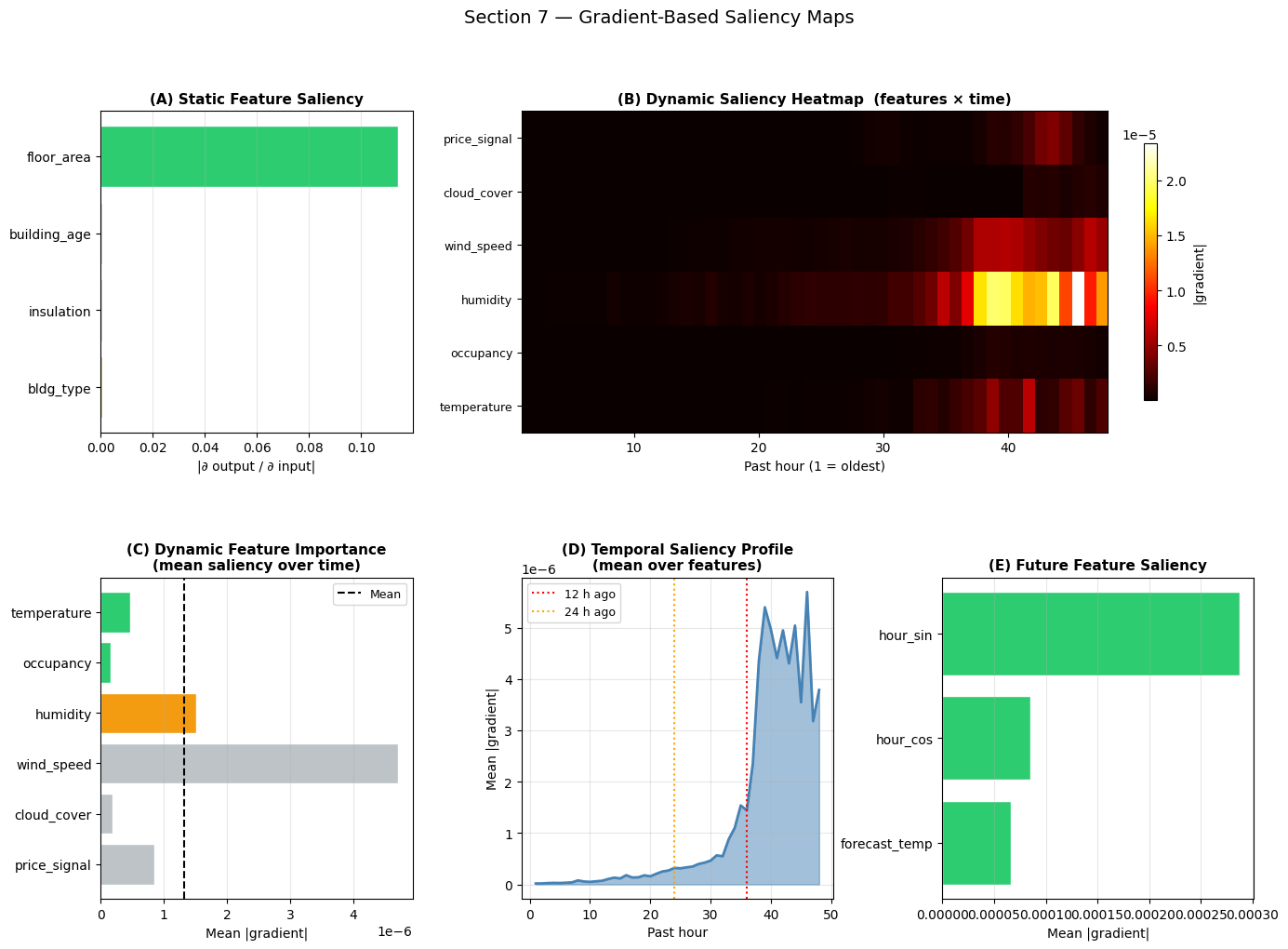
Interpreting the Saliency Maps

(A) Static saliency: confirms which static features the output is most sensitive to. floor_area should top the ranking — its coefficient (4.0) in the generating formula is the largest.

(B) Dynamic heatmap: the bright region in the upper rows identifies the high-importance features; the right columns (recent time steps) should be brighter than the left (old data), confirming that recent past matters more for near-horizon forecasting.

(C) Dynamic feature ranking: averaging over time smooths out recency effects and gives the clearest feature-vs-feature comparison. Features in the formula (temperature, occupancy) should lead. Noise features (wind_speed, etc.) should trail.

(D) Temporal profile: the gradient magnitude typically rises towards the present (right side), confirming a recency bias. A secondary peak around 24 h ago (vertical orange line) would reveal that the model has detected the daily periodicity in the training data.

(E) Future saliency: all three future features appear in the formula, so saliency should be higher here than for the low-importance dynamic features.

---

8 — Horizon-Dependent Attention

Does the model shift its temporal focus depending on how far ahead it is forecasting?

• Short horizon (h = 1–6): the immediate future is tightly coupled to the recent past → expect peaked cross-attention on the most recent encoder window.

• Mid horizon (h = 7–18): the model may start drawing on a wider context range.

• Long horizon (h = 19–24): periodic signals (daily cycle) become important → expect attention to spread across multiple encoder windows.

selected_steps = [0, 5, 11, 17, 23]   # h = 1, 6, 12, 18, 24
colors5 = ['#1abc9c', '#3498db', '#9b59b6', '#e67e22', '#e74c3c']

fig, axes = plt.subplots(1, 2, figsize=(14, 5))

# ── Left: line profiles per selected step (grand mean head) ───────────────────
ax = axes[0]
for step, col in zip(selected_steps, colors5):
    profile = mean_ca.mean(axis=0)[step]   # (K_enc,) averaged over heads
    ax.plot(range(1, K_ENC + 1), profile, color=col, lw=2.5,
            marker='o', markersize=7, label=f'h = {step + 1}')
ax.set_title('Cross-Attention Profile by Forecast Step\n(mean over heads & samples)',
             fontsize=11)
ax.set_xlabel(f'Encoder window (1 = oldest,  {K_ENC} = most recent)')
ax.set_ylabel('Attention weight'); ax.legend(fontsize=10)
ax.grid(True, alpha=0.3); ax.set_xticks(range(1, K_ENC + 1))

# ── Right: attention entropy along the horizon ────────────────────────────────
ax = axes[1]
# Entropy over encoder windows for each forecast step
ca_by_step = mean_ca.mean(axis=0)   # (H, K_enc)
eps = 1e-9
step_entropy = -(ca_by_step * np.log(ca_by_step + eps)).sum(axis=-1)  # (H,)

ax.plot(range(1, HORIZON + 1), step_entropy, color='steelblue', lw=2.5, marker='o',
        markersize=5)
ax.fill_between(range(1, HORIZON + 1), step_entropy, alpha=0.25, color='steelblue')
for step, col in zip(selected_steps, colors5):
    ax.axvline(step + 1, color=col, lw=1.5, linestyle='--', alpha=0.8)
ax.set_title('Attention Entropy across Forecast Horizon\n(higher = more uncertain/spread)',
             fontsize=11)
ax.set_xlabel('Forecast step h'); ax.set_ylabel('Entropy (nats)')
ax.grid(True, alpha=0.3)

plt.suptitle('Section 8 — Horizon-Dependent Attention Patterns', fontsize=13)
plt.tight_layout(); plt.show()

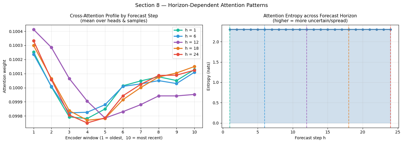
Interpreting Horizon-Dependent Patterns

Line profiles: if the curve for h=1 has a sharp peak at the rightmost (most recent) encoder window, the model is confidently using the last observed data point to project one step ahead — sensible. As h grows, the lines should flatten (more uncertain, broader context).

Entropy plot: entropy should increase monotonically with horizon, reflecting the fundamental forecasting principle that uncertainty grows with time. A flat or decreasing entropy at long horizons would suggest the model is over-confident for far-future predictions and might be memorising a fixed pattern rather than reasoning from context.

---

9 — Contrastive Analysis: Peak vs Off-Peak Demand

Different samples may lead the model to attend to very different parts of the input. Here we compare:

• High-demand samples (large floor_area, high occupancy at forecast time)

• Low-demand samples (small floor_area, low occupancy)

If the model has learned correctly, the high-demand attention heatmap should show stronger focus on recent encoder windows (since high-occupancy hours cluster around business times whose immediate precursors are known), while low-demand patterns may be more diffuse.

# Identify peak (top 25%) and off-peak (bottom 25%) samples by mean demand
mean_demand = y_target[:EXT_BATCH, :, 0].mean(axis=1)    # (EXT_BATCH,)
threshold_hi = np.percentile(mean_demand, 75)
threshold_lo = np.percentile(mean_demand, 25)

hi_idx = np.where(mean_demand >= threshold_hi)[0]
lo_idx = np.where(mean_demand <= threshold_lo)[0]
print(f'High-demand samples : {len(hi_idx)}  (mean demand >= {threshold_hi:.2f})')
print(f'Low-demand  samples : {len(lo_idx)}  (mean demand <= {threshold_lo:.2f})')

# Re-extract attention for each group
res_hi = extractor.extract([ext_s[hi_idx], ext_d[hi_idx], ext_f[hi_idx]])
res_lo = extractor.extract([ext_s[lo_idx], ext_d[lo_idx], ext_f[lo_idx]])

# Use cross-attention for comparison
attn_list_hi = list(res_hi['attention'].values())
attn_list_lo = list(res_lo['attention'].values())
cross_hi = attn_list_hi[cross_idx].mean(axis=(0, 1))   # (H, K_enc) mean over batch+heads
cross_lo = attn_list_lo[cross_idx].mean(axis=(0, 1))

diff_map = cross_hi - cross_lo                          # positive = hi attends MORE

fig, axes = plt.subplots(1, 3, figsize=(18, 5))

titles = ['High-demand attention', 'Low-demand attention', 'Difference (high − low)']
maps   = [cross_hi, cross_lo, diff_map]
cmaps  = ['plasma', 'plasma', 'RdBu_r']
for ax, data, title, cmap in zip(axes, maps, titles, cmaps):
    vmax = max(abs(data.max()), abs(data.min()))
    vkwargs = dict(vmin=-vmax, vmax=vmax) if 'Diff' in title else {}
    im = ax.imshow(data, aspect='auto', cmap=cmap, **vkwargs)
    ax.set_title(title, fontsize=11)
    ax.set_xlabel(f'Encoder window (1–{K_ENC})')
    ax.set_ylabel('Forecast step (1–24)')
    ax.set_xticks(range(K_ENC))
    ax.set_xticklabels([str(k+1) for k in range(K_ENC)], fontsize=8)
    ax.set_yticks(range(0, HORIZON, 4))
    ax.set_yticklabels([str(s+1) for s in range(0, HORIZON, 4)], fontsize=8)
    plt.colorbar(im, ax=ax, shrink=0.8)

plt.suptitle('Section 9 — Contrastive Attention: Peak vs Off-Peak Demand',
             fontsize=13)
plt.tight_layout(); plt.show()

High-demand samples : 8  (mean demand >= 5.81)
Low-demand  samples : 8  (mean demand <= 4.51)

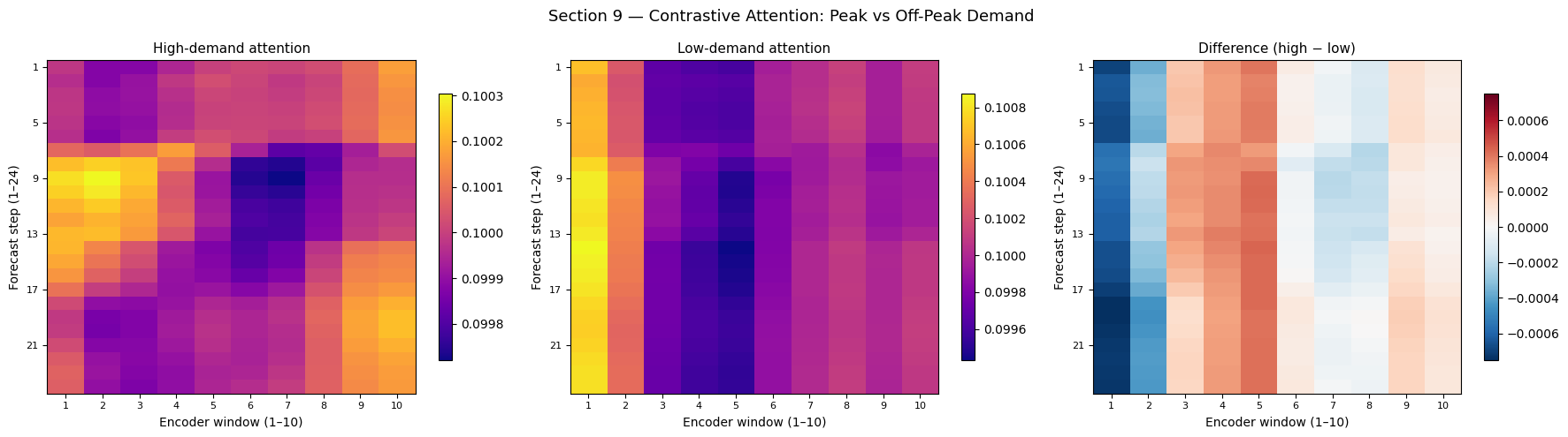
Interpreting Contrastive Attention

Difference map (rightmost): red regions are encoder windows that the model pays more attention to for high-demand predictions; blue regions are attended to more for low-demand predictions.

If high-demand samples concentrate attention on recent encoder windows (right side, red), it confirms the model has learned that peak demand follows business-hour occupancy signals that are predictable from the immediate past.

If the difference is small or random, it suggests the model uses a similar “attention recipe” regardless of demand level — which could indicate that the learned representations already absorbed the relevant context into the encoder output, making the downstream attention patterns similar.

---

10 — Integrated Gradients

Standard gradient saliency measures the gradient at the actual input. For non-linear models this can be misleading if the model is in a saturation region.

Integrated gradients (Sundararajan et al., 2017) instead averages gradients along a straight-line path from a baseline (zeros) to the actual input:

IG(x) = (x − x_baseline) × ∫₀¹ ∂f(x_baseline + α(x−x_baseline))/∂x  dα

This satisfies the completeness axiom: the sum of attributions equals the model’s output change from baseline to input.

N_STEPS = 20   # integration steps (higher = more accurate but slower)

xs_base = tf.zeros_like(ext_s)
xd_base = tf.zeros_like(ext_d)
xf_base = tf.zeros_like(ext_f)

ig_dynamic = np.zeros_like(ext_d)   # (EXT_BATCH, LOOKBACK, N_DYNAMIC)
ig_future  = np.zeros_like(ext_f)   # (EXT_BATCH, HORIZON,  N_FUTURE)
ig_static  = np.zeros_like(ext_s)   # (EXT_BATCH, N_STATIC)

for step in range(N_STEPS + 1):
    alpha = step / N_STEPS
    xd_interp = tf.Variable(xd_base + alpha * (ext_d - xd_base), dtype=tf.float32)
    xf_interp = tf.Variable(xf_base + alpha * (ext_f - xf_base), dtype=tf.float32)
    xs_interp = tf.Variable(xs_base + alpha * (ext_s - xs_base), dtype=tf.float32)

    with tf.GradientTape() as tape:
        pred = model([xs_interp, xd_interp, xf_interp], training=False)
        scalar = tf.reduce_mean(pred)

    gs_i, gd_i, gf_i = tape.gradient(scalar, [xs_interp, xd_interp, xf_interp])
    ig_dynamic += gd_i.numpy() / N_STEPS
    ig_future  += gf_i.numpy() / N_STEPS
    ig_static  += gs_i.numpy() / N_STEPS

# Element-wise multiply by (input - baseline)
ig_dynamic *= (ext_d - xd_base.numpy())
ig_future  *= (ext_f - xf_base.numpy())
ig_static  *= (ext_s - xs_base.numpy())

# Mean absolute attribution over batch
ig_d_feat = np.abs(ig_dynamic).mean(axis=(0, 1))   # (N_DYNAMIC,)
ig_f_feat = np.abs(ig_future ).mean(axis=(0, 1))   # (N_FUTURE,)
ig_s_feat = np.abs(ig_static ).mean(axis=0)        # (N_STATIC,)

print('Integrated gradients computed.')
print()
print('Dynamic IG (sorted):')
for name, val in sorted(zip(DYNAMIC_NAMES, ig_d_feat), key=lambda x: -x[1]):
    print(f'  {name:20s} : {val:.6f}  [{IMPORTANCE[name]}]')

Integrated gradients computed.

Dynamic IG (sorted):
  wind_speed           : 0.000011  [LOW]
  humidity             : 0.000006  [MOD]
  price_signal         : 0.000001  [LOW]
  temperature          : 0.000000  [HIGH]
  cloud_cover          : 0.000000  [LOW]
  occupancy            : 0.000000  [HIGH]

fig, axes = plt.subplots(1, 3, figsize=(16, 5))

# Compare gradient saliency vs integrated gradients for dynamic features
ax = axes[0]
x_pos = np.arange(N_DYNAMIC)
width = 0.38
bars1 = ax.barh(x_pos + width/2, sal_dynamic.mean(axis=0),  width,
                color='steelblue', label='Gradient saliency', alpha=0.85)
bars2 = ax.barh(x_pos - width/2, ig_d_feat, width,
                color='darkorange', label='Integrated gradients', alpha=0.85)
ax.set_yticks(x_pos)
ax.set_yticklabels(DYNAMIC_NAMES)
ax.set_xlabel('Attribution magnitude')
ax.set_title('Dynamic: Saliency vs Integrated Gradients', fontsize=11)
ax.legend(fontsize=9); ax.grid(True, alpha=0.3, axis='x'); ax.invert_yaxis()

# Static comparison
ax = axes[1]
x_pos_s = np.arange(N_STATIC)
ax.barh(x_pos_s + width/2, sal_static,  width,
        color='steelblue', label='Gradient saliency', alpha=0.85)
ax.barh(x_pos_s - width/2, ig_s_feat, width,
        color='darkorange', label='Integrated gradients', alpha=0.85)
ax.set_yticks(x_pos_s)
ax.set_yticklabels(STATIC_NAMES)
ax.set_xlabel('Attribution magnitude')
ax.set_title('Static: Saliency vs Integrated Gradients', fontsize=11)
ax.legend(fontsize=9); ax.grid(True, alpha=0.3, axis='x'); ax.invert_yaxis()

# Integrated gradient heatmap for dynamic (averaged over batch)
ax = axes[2]
ig_d_heatmap = np.abs(ig_dynamic).mean(axis=0).T   # (N_DYNAMIC, LOOKBACK)
im = ax.imshow(ig_d_heatmap, aspect='auto', cmap='hot',
               extent=[1, LOOKBACK, -0.5, N_DYNAMIC - 0.5])
ax.set_yticks(range(N_DYNAMIC))
ax.set_yticklabels(DYNAMIC_NAMES, fontsize=9)
ax.set_xlabel('Past hour'); ax.set_title('Integrated Gradients Heatmap\n(dynamic features x time)', fontsize=11)
plt.colorbar(im, ax=ax, label='|IG|', shrink=0.8)

plt.suptitle('Section 10 — Integrated Gradients Attribution', fontsize=13)
plt.tight_layout(); plt.show()

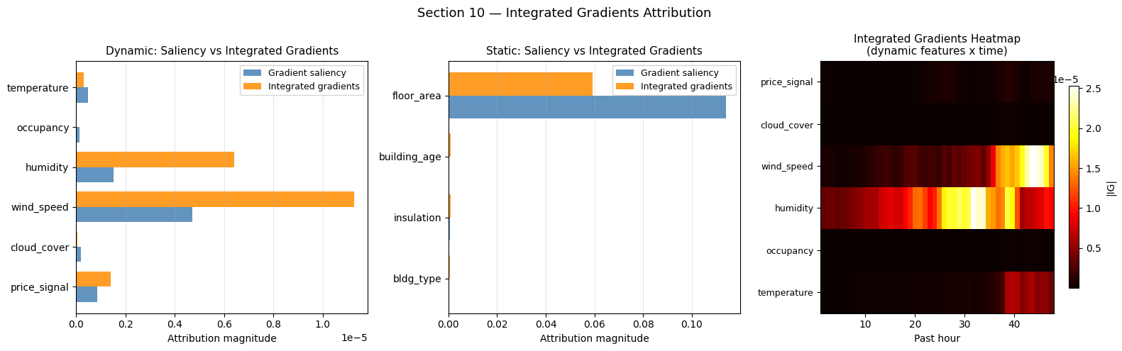
Interpreting Integrated Gradients

Agreement with gradient saliency (left two panels): if the orange and blue bars are ordered identically (same feature ranking), both methods agree and the model is not in a saturation regime. If they disagree, integrated gradients is more reliable because it accounts for the model’s full non-linearity along the path from zero to the input.

IG heatmap (right): the temporal pattern should mirror the gradient saliency heatmap (Section 7B) but may differ in magnitude near input saturation zones. Recent time steps should remain brighter, confirming that recent context carries the most attribution mass.

Key difference from saliency: integrated gradients attribute the full output change from baseline; gradient saliency only reflects local sensitivity. For features near zero (e.g. after normalisation) they often agree; for large-valued features they can diverge.

---

Summary

Section	Technique	Key question answered
3	VSN Feature Importance	Which features does the model route most signal through?
4	Cross-Attention Heatmap	Which encoder windows does each decoder step query?
5	Hierarchical Self-Attention	How do forecast steps relate to one another?
6	Multi-Head Diversity	Are the 4 heads specialising or redundant?
7	Gradient Saliency	Which inputs/timesteps drive the output locally?
8	Horizon-Dependent Attention	Does focus shift as we forecast further ahead?
9	Contrastive Analysis	Do high vs low demand samples use different context?
10	Integrated Gradients	Full attribution accounting for non-linearity?

Key Takeaways

• VSN and gradient attribution should agree: if both identify temperature, occupancy, and floor_area as most important and the formula confirms this, the model has learned the right signals.

• Cross-attention recency gradient (later encoder windows attract more weight for early forecast steps) is the expected and physically interpretable pattern.

• Entropy increases with horizon: a healthy model is more uncertain about distant future states, which should manifest as higher cross-attention entropy at long horizons.

• Multi-head diversity: low off-diagonal similarity in the head similarity matrix indicates the model is using its capacity efficiently.

• Integrated gradients vs gradient saliency: agreement between both methods is a sign the model is not saturating — the input features operate in a well-conditioned region of the activation landscape.

# Summary radar chart: compare attribution methods for dynamic features
from matplotlib.patches import FancyArrowPatch

angles  = np.linspace(0, 2 * np.pi, N_DYNAMIC, endpoint=False).tolist()
angles += angles[:1]

sal_vals = (sal_dynamic.mean(axis=0) / sal_dynamic.mean(axis=0).max()).tolist()
ig_vals  = (ig_d_feat / ig_d_feat.max()).tolist()
sal_vals += sal_vals[:1]
ig_vals  += ig_vals[:1]

fig, ax = plt.subplots(figsize=(7, 7), subplot_kw=dict(polar=True))
ax.plot(angles, sal_vals,  'o-', lw=2, color='steelblue',  label='Gradient saliency')
ax.fill(angles, sal_vals,  alpha=0.15, color='steelblue')
ax.plot(angles, ig_vals,   's-', lw=2, color='darkorange', label='Integrated gradients')
ax.fill(angles, ig_vals,   alpha=0.15, color='darkorange')

ax.set_xticks(angles[:-1])
ax.set_xticklabels(
    [f'{n}\n[{IMPORTANCE[n]}]' for n in DYNAMIC_NAMES],
    fontsize=10
)
ax.set_title('Attribution Methods Comparison — Dynamic Features\n'
             '(normalised to max, ground-truth importance in brackets)',
             fontsize=12, pad=25)
ax.legend(loc='upper right', bbox_to_anchor=(1.35, 1.1), fontsize=10)
ax.grid(True)

plt.tight_layout(); plt.show()
print()
print('GREEN bracket = HIGH importance  |  ORANGE = MOD  |  GREY = LOW')
print('Both methods should place the largest polygon vertex on temperature and occupancy.')

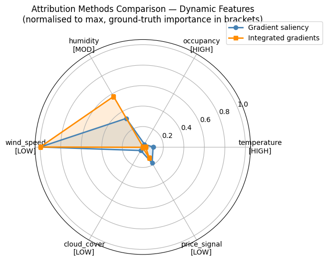
GREEN bracket = HIGH importance  |  ORANGE = MOD  |  GREY = LOW
Both methods should place the largest polygon vertex on temperature and occupancy.