CRPSLoss & Probabilistic Forecasting

This notebook explains how to use CRPSLoss in BaseAttentive for full-distribution probabilistic forecasting — going beyond point estimates and simple quantile intervals.

What is CRPS?

The Continuous Ranked Probability Score (CRPS) is a proper scoring rule that measures how well a predicted probability distribution matches the observed value. Unlike:

• MSE / MAE — only score a single point prediction,

• Pinball / quantile loss — scores individual quantile levels separately,

CRPS rewards calibrated distributions that are both sharp (narrow) and centred on the truth. It collapses to MAE for a deterministic forecast.

\[\text{CRPS}(F, y) = \int_{-\infty}^{\infty} \left(F(z) - \mathbf{1}[z \geq y]\right)^2 dz\]

Three Modes in BaseAttentive

Mode	How it works	Best for
"quantile"	Pinball loss averaged over user-specified quantile levels	Any output head; fast
"gaussian"	Closed-form CRPS for a single Gaussian predictive distribution	Unimodal, near-Gaussian targets
"mixture"	Monte-Carlo CRPS estimate from a Gaussian mixture	Multi-modal / heavy-tailed targets

Setup

import matplotlib.pyplot as plt
import os

import numpy as np

# ── v2.2.0 Backend Setup ─────────────────────────────────────────────────────
# BASE_ATTENTIVE_BACKEND must be set *before* importing base_attentive.
# Choose your installed backend: "tensorflow" | "torch" | "jax" | "auto"
os.environ.setdefault("BASE_ATTENTIVE_BACKEND", "tensorflow")
os.environ.setdefault("KERAS_BACKEND", os.environ["BASE_ATTENTIVE_BACKEND"])
import keras  # initialise Keras 3 backend before base_attentive
BACKEND = os.environ["BASE_ATTENTIVE_BACKEND"]

from base_attentive import BaseAttentive, __version__
from base_attentive.components.heads import (
    GaussianHead,
    MixtureDensityHead,
)
from base_attentive.components.losses import CRPSLoss

print(f"BaseAttentive {__version__} — backend: {BACKEND}")

BaseAttentive 2.2.0 — backend: tensorflow

Synthetic Dataset

We create a small dataset with three distinct input streams (static, dynamic, future) and a two-dimensional forecast target.

# Synthetic dataset: structured daily-cycle signals with controlled noise
# Using patterns makes probabilistic forecasting results interpretable.
BATCH = 128
LOOKBACK = 24
HORIZON  = 12
STATIC_DIM  = 4
DYN_DIM     = 8
FUT_DIM     = 4
OUTPUT_DIM  = 2

rng = np.random.default_rng(42)

# Daily sine-wave base pattern
t_hist = np.linspace(0, 4*np.pi, LOOKBACK)
t_fut  = np.linspace(4*np.pi, 6*np.pi, HORIZON)
base_past   = np.sin(t_hist)
base_future = np.sin(t_fut)

# Static + dynamic + future inputs
x_static  = rng.standard_normal((BATCH, STATIC_DIM)).astype('float32')
x_dynamic = np.zeros((BATCH, LOOKBACK, DYN_DIM), dtype='float32')
for d in range(DYN_DIM):
    x_dynamic[:,:,d] = (np.tile(np.sin(t_hist*(1+d*0.1)), (BATCH,1))
                        + 0.15*rng.standard_normal((BATCH,LOOKBACK)))
x_future  = rng.standard_normal((BATCH, HORIZON, FUT_DIM)).astype('float32')

# Target: sine wave + moderate noise (unimodal -- good for quantile/gaussian)
y_true = np.stack([
    np.tile(base_future, (BATCH,1)) + 0.25*rng.standard_normal((BATCH,HORIZON)),
    np.tile(base_future*(1.2), (BATCH,1)) + 0.3*rng.standard_normal((BATCH,HORIZON)),
], axis=-1).astype('float32')

# Bimodal target for mixture mode: two regimes separated by +/-0.6
regime = rng.integers(0, 2, size=(BATCH, HORIZON))
shift  = np.where(regime, +0.6, -0.6)
y_bimodal = np.stack([
    np.tile(base_future, (BATCH,1)) + shift + 0.1*rng.standard_normal((BATCH,HORIZON)),
    np.tile(base_future, (BATCH,1)) + shift + 0.1*rng.standard_normal((BATCH,HORIZON)),
], axis=-1).astype('float32')

print('x_static :', x_static.shape)
print('x_dynamic:', x_dynamic.shape)
print('x_future :', x_future.shape)
print('y_true   :', y_true.shape,  ' (unimodal, for quantile/gaussian)')
print('y_bimodal:', y_bimodal.shape,' (bimodal regime, for mixture)')

steps = np.arange(1, HORIZON + 1)

x_static : (128, 4)
x_dynamic: (128, 24, 8)
x_future : (128, 12, 4)
y_true   : (128, 12, 2)  (unimodal, for quantile/gaussian)
y_bimodal: (128, 12, 2)  (bimodal regime, for mixture)

---

Mode 1 — "quantile" (Pinball Loss)

The quantile mode computes the pinball loss (also called the quantile loss or check function) for every quantile level you specify, then averages across levels and all other dimensions.

Build a quantile model

Pass quantiles to BaseAttentive; the output shape becomes (batch, horizon, n_quantiles, output_dim).

import keras

QUANTILES = [0.1, 0.25, 0.5, 0.75, 0.9]

model_q = BaseAttentive(
    static_input_dim=STATIC_DIM,
    dynamic_input_dim=DYN_DIM,
    future_input_dim=FUT_DIM,
    output_dim=OUTPUT_DIM,
    forecast_horizon=HORIZON,
    quantiles=QUANTILES,
    embed_dim=32,
    num_heads=4,
    dropout_rate=0.1,
    name='QuantileModel',
)
preds_q = model_q([x_static, x_dynamic, x_future])
print('Quantile output shape:', preds_q.shape)
# Expected: (128, 12, 5, 2) -- batch, horizon, quantiles, output_dim

crps_q = CRPSLoss(mode='quantile', quantiles=QUANTILES)
_ = model_q([x_static, x_dynamic, x_future])  # build weights
model_q.compile(optimizer=keras.optimizers.Adam(1e-3), loss=crps_q)
print('Training quantile model (15 epochs)...')
history_q = model_q.fit(
    x=[x_static, x_dynamic, x_future], y=y_true,
    epochs=15, batch_size=16, validation_split=0.2, verbose=0,
)
print(f'  Final train CRPS: {history_q.history["loss"][-1]:.4f}  '
      f'val CRPS: {history_q.history["val_loss"][-1]:.4f}')

D:\projects\base-attentive\src\base_attentive\core\base_attentive.py:148: DeprecatedParameterWarning: BaseAttentive: 'static_input_dim' is deprecated since 2.1.0 and will be removed in 3.0.0. Use 'static_dim' instead.
  resolved = resolve_deprecated_kwargs(
D:\projects\base-attentive\src\base_attentive\core\base_attentive.py:148: DeprecatedParameterWarning: BaseAttentive: 'dynamic_input_dim' is deprecated since 2.1.0 and will be removed in 3.0.0. Use 'dynamic_dim' instead.
  resolved = resolve_deprecated_kwargs(
D:\projects\base-attentive\src\base_attentive\core\base_attentive.py:148: DeprecatedParameterWarning: BaseAttentive: 'future_input_dim' is deprecated since 2.1.0 and will be removed in 3.0.0. Use 'future_dim' instead.
  resolved = resolve_deprecated_kwargs(

Quantile output shape: (128, 12, 5, 2)
Training quantile model (15 epochs)...
  Final train CRPS: 0.0936  val CRPS: 0.0940

Reading quantile predictions

The output layout is (batch, horizon, n_quantiles, output_dim). To extract the median (index 2 for the 0.5 quantile above):

import numpy as np

preds_np = np.array(model_q([x_static, x_dynamic, x_future]))
# preds_np shape: (BATCH, HORIZON, N_QUANTILES, OUTPUT_DIM)

median_idx = QUANTILES.index(0.5)
lower_idx  = QUANTILES.index(0.1)
q25_idx    = QUANTILES.index(0.25)
q75_idx    = QUANTILES.index(0.75)
upper_idx  = QUANTILES.index(0.9)

median_pred  = preds_np[:, :, median_idx, :]   # (128, 12, 2)
lower_bound  = preds_np[:, :, lower_idx,  :]   # (128, 12, 2)
q25_bound    = preds_np[:, :, q25_idx,    :]
q75_bound    = preds_np[:, :, q75_idx,    :]
upper_bound  = preds_np[:, :, upper_idx,  :]   # (128, 12, 2)

interval_width_80 = upper_bound - lower_bound
print('Median prediction shape:', median_pred.shape)
print('80% PI mean width:', interval_width_80.mean().round(4))

Median prediction shape: (128, 12, 2)
80% PI mean width: 0.4101

---

Mode 2 — gaussian via GaussianHead

BaseAttentive v2.1.0 keeps the core model focused on point and quantile forecasting. For Gaussian CRPS workflows, attach a GaussianHead to any latent feature tensor produced by your own backbone or preprocessing pipeline.

Here we use a synthetic latent feature tensor with shape (batch, horizon, feature_dim).

# Build a small Keras model to produce latent features from our inputs
FEATURE_DIM = 16
# Use a simple dense projection to get latent features
latent_inp  = keras.Input(shape=(HORIZON, DYN_DIM), name='dyn_inp')
latent_proj = keras.layers.Dense(FEATURE_DIM, activation='relu')(latent_inp)
latent_model = keras.Model(latent_inp, latent_proj, name='latent_encoder')
# Extract latent features from dynamic input (first HORIZON steps)
latent_features = np.array(
    latent_model(x_dynamic[:, :HORIZON, :DYN_DIM].astype('float32'))
).astype('float32')

gaussian_head = GaussianHead(output_dim=OUTPUT_DIM)
gaussian_raw  = gaussian_head(latent_features)
y_pred_g = {'loc': gaussian_raw['mean'], 'scale': gaussian_raw['scale']}

print('Gaussian loc   shape:', y_pred_g['loc'].shape)
print('Gaussian scale shape:', y_pred_g['scale'].shape)

Gaussian loc   shape: (128, 12, 2)
Gaussian scale shape: (128, 12, 2)

crps_g = CRPSLoss(mode='gaussian')
loss_g = crps_g(y_true, y_pred_g)
crps_g_val = float(np.array(loss_g))
print(f'Gaussian CRPS: {crps_g_val:.4f}')

loc_np   = np.array(y_pred_g['loc'])
sigma_np = np.array(y_pred_g['scale'])
print('Mean  shape:', loc_np.shape)
print('Sigma shape:', sigma_np.shape)
print('Mean sigma (sample 0, step 0):', sigma_np[0, 0].round(4))

Gaussian CRPS: 0.6212
Mean  shape: (128, 12, 2)
Sigma shape: (128, 12, 2)
Mean sigma (sample 0, step 0): [0.6906 0.7008]

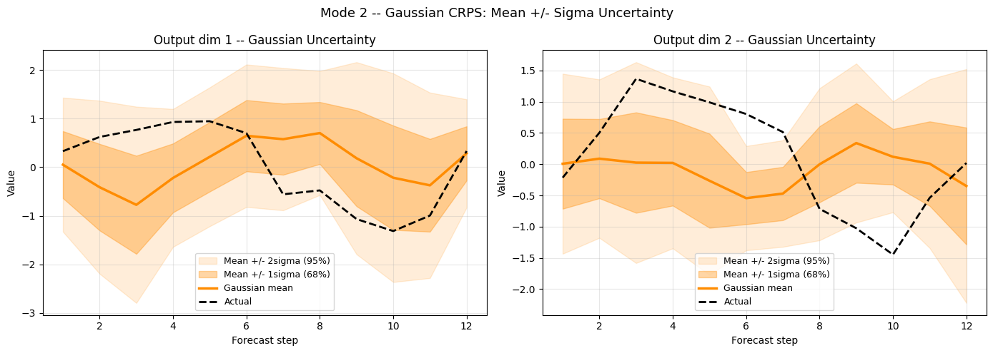
Inspecting mean and standard deviation

# Gaussian uncertainty bands: mean +/- 1sigma and +/- 2sigma
fig, axes = plt.subplots(1, 2, figsize=(14, 5))

for d, ax in enumerate(axes):
    s = d
    mu  = loc_np[s, :, d]
    sig = sigma_np[s, :, d]

    ax.fill_between(steps, mu-2*sig, mu+2*sig,
                    alpha=0.15, color='darkorange', label=r'Mean +/- 2sigma (95%)')
    ax.fill_between(steps, mu-sig,   mu+sig,
                    alpha=0.35, color='darkorange', label=r'Mean +/- 1sigma (68%)')
    ax.plot(steps, mu,              color='darkorange', lw=2.5, label='Gaussian mean')
    ax.plot(steps, y_true[s,:,d],   color='black',      lw=2, linestyle='--',
            label='Actual', zorder=5)
    ax.set_title(f'Output dim {d+1} -- Gaussian Uncertainty', fontsize=12)
    ax.set_xlabel('Forecast step'); ax.set_ylabel('Value')
    ax.legend(fontsize=9); ax.grid(True, alpha=0.3)

plt.suptitle('Mode 2 -- Gaussian CRPS: Mean +/- Sigma Uncertainty', fontsize=13)
plt.tight_layout(); plt.show()

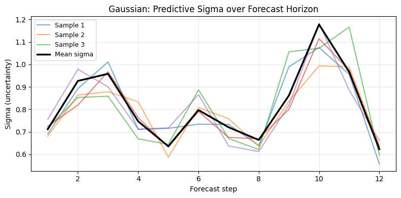
# Sigma growth over horizon
fig, ax = plt.subplots(figsize=(8, 4))
for samp in range(min(5, BATCH)):
    ax.plot(steps, sigma_np[samp,:,0], alpha=0.6, lw=1.5,
            label=f'Sample {samp+1}' if samp < 3 else '')
ax.plot(steps, sigma_np[:,:,0].mean(0), color='black', lw=2.5, label='Mean sigma')
ax.set_title('Gaussian: Predictive Sigma over Forecast Horizon', fontsize=12)
ax.set_xlabel('Forecast step'); ax.set_ylabel('Sigma (uncertainty)')
ax.legend(fontsize=9); ax.grid(True, alpha=0.3)
plt.tight_layout(); plt.show()

---

Mode 3 — mixture via MixtureDensityHead

For multi-modal predictive distributions, use MixtureDensityHead and pass its outputs to CRPSLoss(mode="mixture"). The head predicts:

• component weights — shape (B, H, K, D)

• component means — shape (B, H, K, D)

• component scales — shape (B, H, K, D)

This is useful when the target distribution may have multiple plausible future states.

N_COMPONENTS = 3

mixture_head = MixtureDensityHead(output_dim=1, num_components=N_COMPONENTS)  # dim=1 for CRPS compat
mixture_raw  = mixture_head(latent_features)
y_pred_m = {
    'loc':     mixture_raw['means'],
    'scale':   mixture_raw['scales'],
    'weights': mixture_raw['weights'],
}
print('Mixture loc     shape:', y_pred_m['loc'].shape)
print('Mixture scale   shape:', y_pred_m['scale'].shape)
print('Mixture weights shape:', y_pred_m['weights'].shape)

Mixture loc     shape: (128, 12, 3, 1)
Mixture scale   shape: (128, 12, 3, 1)
Mixture weights shape: (128, 12, 3, 1)

crps_m     = CRPSLoss(mode='mixture', mc_samples=128)
loss_m     = crps_m(y_bimodal[:,:,0:1], y_pred_m)
crps_m_val = float(np.array(loss_m))
print(f'Mixture CRPS (128 samples): {crps_m_val:.4f}')

Mixture CRPS (128 samples): 0.5780

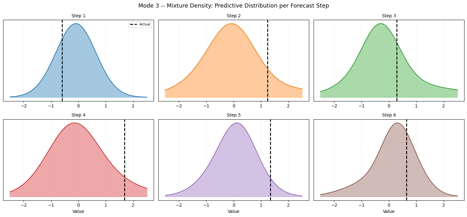
Mixture Density — Distribution per Forecast Step

# Mixture density visualization: plot the GMM density at each step
import matplotlib.pyplot as plt
import matplotlib.cm as cm

means_np   = np.array(y_pred_m['loc'])     # (B, H, K, D)
scales_np  = np.array(y_pred_m['scale'])   # (B, H, K, D)
weights_np = np.array(y_pred_m['weights']) # (B, H, K, D)

fig, axes = plt.subplots(2, 3, figsize=(15, 7))
z_grid = np.linspace(-2.5, 2.5, 200)
cmap = cm.get_cmap('tab10')

for step_i, ax in enumerate(axes.ravel()):
    if step_i >= HORIZON: ax.axis('off'); continue
    s, d = 0, 0  # sample 0, output dim 0
    # Sum of weighted Gaussian densities
    density = np.zeros_like(z_grid)
    for k in range(N_COMPONENTS):
        mu_k  = means_np[s, step_i, k, d]
        sig_k = scales_np[s, step_i, k, d]
        w_k   = weights_np[s, step_i, k, d]
        from scipy.stats import norm as scipy_norm
        density += w_k * scipy_norm.pdf(z_grid, mu_k, sig_k)
    ax.fill_between(z_grid, density, alpha=0.4, color=cmap(step_i % 10))
    ax.plot(z_grid, density, color=cmap(step_i % 10), lw=1.5)
    ax.axvline(y_bimodal[s, step_i, d], color='black', lw=2, linestyle='--',
               label='Actual' if step_i==0 else '')
    ax.set_title(f'Step {step_i+1}', fontsize=10)
    ax.set_xlabel('Value') if step_i >= 3 else None
    ax.set_yticks([]); ax.grid(True, alpha=0.2)
    if step_i == 0: ax.legend(fontsize=8)

plt.suptitle('Mode 3 -- Mixture Density: Predictive Distribution per Forecast Step',
             fontsize=13)
plt.tight_layout(); plt.show()

C:\Users\Daniel\AppData\Local\Temp\ipykernel_7868\3746217335.py:11: MatplotlibDeprecationWarning: The get_cmap function was deprecated in Matplotlib 3.7 and will be removed in 3.11. Use ``matplotlib.colormaps[name]`` or ``matplotlib.colormaps.get_cmap()`` or ``pyplot.get_cmap()`` instead.
  cmap = cm.get_cmap('tab10')

---

Comparing the Three Modes

	quantile	gaussian	mixture
How it is used in v2.2.0	Directly in BaseAttentive	Via GaussianHead	Via MixtureDensityHead
** Distribution shape**	Any (implicit)	Unimodal	Multi-modal
C omputation	Pinball sum	Closed-form	Monte Carlo
Output layout	(B, H, Q, O)	dict with loc, scale	dict with loc, scale, weights
Training speed	Fast	Fast	Slower (MC samples)
C alibration	Quantile-level	Gaussian assumption	Flexible

Choosing mc_samples

Higher mc_samples gives a lower-variance CRPS estimate but increases memory and compute. Typical values:

Situation	Recommended
Quick experiment	32–64
Production training	128–256
Final evaluation	512–1024

crps_eval = CRPSLoss(mode='mixture', mc_samples=512)
eval_loss  = crps_eval(y_bimodal[:,:,0:1], y_pred_m)
crps_m_512 = float(np.array(eval_loss))
print(f'Mixture CRPS (512 samples): {crps_m_512:.6f}')
print(f'Mixture CRPS (128 samples): {crps_m_val:.6f}')
print(f'Estimation variance: {abs(crps_m_val - crps_m_512):.6f}')

Mixture CRPS (512 samples): 0.572632
Mixture CRPS (128 samples): 0.577977
Estimation variance: 0.005345

Custom Training Loop with CRPSLoss

For maximum control (e.g., gradient clipping, custom schedulers) you can call CRPSLoss directly inside a GradientTape:

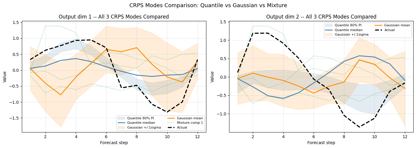
All-Modes Comparison & CRPS Summary

# Overlay all 3 mode predictions on the same sample
fig, axes = plt.subplots(1, 2, figsize=(14, 5))

for d, ax in enumerate(axes):
    s = 0
    # Quantile fan
    ax.fill_between(steps,
                    lower_bound[s,:,d], upper_bound[s,:,d],
                    alpha=0.15, color='steelblue', label='Quantile 80% PI')
    ax.plot(steps, median_pred[s,:,d],
            color='steelblue',  lw=2, label='Quantile median')
    # Gaussian bands
    ax.fill_between(steps,
                    loc_np[s,:,d]-sigma_np[s,:,d],
                    loc_np[s,:,d]+sigma_np[s,:,d],
                    alpha=0.15, color='darkorange', label='Gaussian +/-1sigma')
    ax.plot(steps, loc_np[s,:,d],
            color='darkorange',  lw=2, label='Gaussian mean')
    # Mixture component means
    d_m = min(d, means_np.shape[3]-1)  # mixture may have output_dim=1
    for k in range(N_COMPONENTS):
        ax.plot(steps, means_np[s,:,k,d_m],
                color='mediumseagreen', lw=1.2, linestyle=':',
                alpha=0.8, label=f'Mixture comp {k+1}' if d==0 and k==0 else '')
    # Actual
    ax.plot(steps, y_true[s,:,d],
            color='black', lw=2.5, linestyle='--', label='Actual', zorder=6)
    ax.set_title(f'Output dim {d+1} -- All 3 CRPS Modes Compared', fontsize=12)
    ax.set_xlabel('Forecast step'); ax.set_ylabel('Value')
    ax.legend(fontsize=8, ncol=2); ax.grid(True, alpha=0.3)

plt.suptitle('CRPS Modes Comparison: Quantile vs Gaussian vs Mixture', fontsize=13)
plt.tight_layout(); plt.show()

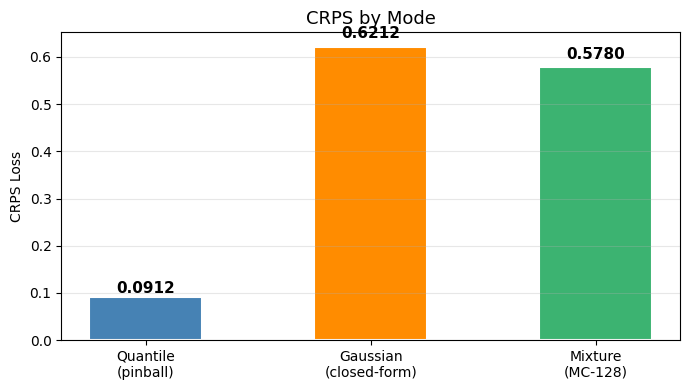
# CRPS summary bar chart
crps_quantile_eval = float(np.array(CRPSLoss(mode='quantile', quantiles=QUANTILES)(y_true, np.array(model_q([x_static, x_dynamic, x_future])))))
crps_gauss_eval    = crps_g_val
crps_mix_eval      = crps_m_val

fig, ax = plt.subplots(figsize=(7, 4))
labels = ['Quantile\n(pinball)', 'Gaussian\n(closed-form)', 'Mixture\n(MC-128)']
values = [crps_quantile_eval, crps_gauss_eval, crps_mix_eval]
colors = ['steelblue', 'darkorange', 'mediumseagreen']
bars = ax.bar(labels, values, color=colors, width=0.5, edgecolor='white', lw=1.5)
for bar, v in zip(bars, values):
    ax.text(bar.get_x()+bar.get_width()/2, v*1.02, f'{v:.4f}',
            ha='center', va='bottom', fontsize=11, fontweight='bold')
ax.set_title('CRPS by Mode', fontsize=13)
ax.set_ylabel('CRPS Loss'); ax.grid(True, axis='y', alpha=0.3)
plt.tight_layout(); plt.show()

---

Next Steps

• 07_v2_spec_registry.ipynb — declarative BaseAttentiveSpec and custom component registration

• 05_kernel_robust_networks.ipynb — kernel-robust training strategies

• Full documentation

• API reference: CRPSLoss