BaseAttentive Standalone Applications
This notebook demonstrates practical applications of BaseAttentive as a standalone time series forecasting model for various real-world scenarios.
Table of Contents
Air Quality Forecasting
Energy Demand Forecasting
Weather Prediction
Traffic Flow Prediction
Setup and Imports
[1]:
import os
import warnings

import numpy as np

warnings.filterwarnings("ignore")

# ── v2.2.0 Backend Setup ─────────────────────────────────────────────────────
# BASE_ATTENTIVE_BACKEND must be set *before* importing base_attentive.
# Choose your installed backend: "tensorflow" | "torch" | "jax" | "auto"
os.environ.setdefault("BASE_ATTENTIVE_BACKEND", "tensorflow")
os.environ.setdefault("KERAS_BACKEND", os.environ["BASE_ATTENTIVE_BACKEND"])
import keras  # initialise Keras 3 backend before base_attentive
BACKEND = os.environ["BASE_ATTENTIVE_BACKEND"]

from base_attentive import BaseAttentive, __version__

print(f"BaseAttentive {__version__} — backend: {BACKEND}")
BaseAttentive 2.2.0 — backend: tensorflow
1. Air Quality Forecasting
Use Case
Predict PM2.5 air pollution levels based on:
Static features: Location (latitude, longitude), altitude, urban/rural indicator
Dynamic past features: Historical PM2.5, NO₂, O₃, temperature, humidity
Known future features: Forecasted wind speed, temperature
Application
Public health alerts
Air quality advisories
Industrial emission controls
[2]:
# Air Quality -- realistic PM2.5 with daily rush-hour pattern
np.random.seed(42)
N_AIR, LOOKBACK_AIR, HORIZON_AIR = 128, 72, 24

def pm25_profile(t):
    morning = 22 * np.exp(-0.5 * ((t % 24 - 8)  / 1.5) ** 2)
    evening = 18 * np.exp(-0.5 * ((t % 24 - 18) / 2.0) ** 2)
    return (20 + morning + evening).astype('float32')

t_buf = np.arange(LOOKBACK_AIR + HORIZON_AIR + 24)
base  = pm25_profile(t_buf)
offsets = np.random.randint(0, 24, N_AIR)

pm25_past   = np.array([base[o : o+LOOKBACK_AIR]                           for o in offsets])
pm25_future = np.array([base[o+LOOKBACK_AIR : o+LOOKBACK_AIR+HORIZON_AIR] for o in offsets])

static_features = np.random.randn(N_AIR, 4).astype('float32')
static_features[:, 2] = np.abs(static_features[:, 2]) * 1000
static_features[:, 3] = (static_features[:, 3] > 0).astype('float32')

dynamic_past = np.zeros((N_AIR, LOOKBACK_AIR, 5), dtype='float32')
dynamic_past[:,:,0] = pm25_past + np.random.randn(N_AIR, LOOKBACK_AIR).astype('float32') * 3
dynamic_past[:,:,1] = np.abs(np.random.randn(N_AIR, LOOKBACK_AIR)).astype('float32') * 40
dynamic_past[:,:,2] = np.abs(np.random.randn(N_AIR, LOOKBACK_AIR)).astype('float32') * 25
dynamic_past[:,:,3] = 15 + np.random.randn(N_AIR, LOOKBACK_AIR).astype('float32') * 5
dynamic_past[:,:,4] = 55 + np.abs(np.random.randn(N_AIR, LOOKBACK_AIR)).astype('float32') * 18

known_future = np.zeros((N_AIR, HORIZON_AIR, 2), dtype='float32')
known_future[:,:,0] = np.abs(np.random.randn(N_AIR, HORIZON_AIR)).astype('float32') * 3
known_future[:,:,1] = 15 + np.random.randn(N_AIR, HORIZON_AIR).astype('float32') * 4

target = np.clip(
    pm25_future + np.random.randn(N_AIR, HORIZON_AIR).astype('float32') * 3, 0, 150
)[:, :, None]

print('Air Quality Data Shapes:')
for nm, a in [('Static',static_features),('Dynamic',dynamic_past),
              ('Future',known_future),('Target PM2.5',target)]:
    print(f'  {nm:14s}: {a.shape}')
print(f'  PM2.5 past [{dynamic_past[:,:,0].min():.1f}, {dynamic_past[:,:,0].max():.1f}]  '
      f'target [{target.min():.1f}, {target.max():.1f}] ug/m3')
Air Quality Data Shapes:
  Static        : (128, 4)
  Dynamic       : (128, 72, 5)
  Future        : (128, 24, 2)
  Target PM2.5  : (128, 24, 1)
  PM2.5 past [8.9, 50.3]  target [9.8, 48.8] ug/m3
[3]:
import keras

air_quality_model = BaseAttentive(
    static_input_dim=4, dynamic_input_dim=5, future_input_dim=2,
    output_dim=1, forecast_horizon=HORIZON_AIR,
    objective='hybrid',
    architecture_config={'decoder_attention_stack': ['cross', 'hierarchical']},
    embed_dim=32, num_heads=4, dropout_rate=0.1, name='air_quality_model',
)
_ = air_quality_model([static_features, dynamic_past, known_future])  # build weights
air_quality_model.compile(optimizer=keras.optimizers.Adam(1e-3), loss='mse', metrics=['mae'])
print('Training air quality model (15 epochs)...')
history_air = air_quality_model.fit(
    [static_features, dynamic_past, known_future], target,
    epochs=15, batch_size=16, validation_split=0.2, verbose=0,
)
print(f'  train_MSE={history_air.history["loss"][-1]:.3f}  '
      f'val_MSE={history_air.history["val_loss"][-1]:.3f}  '
      f'val_MAE={history_air.history["val_mae"][-1]:.2f} ug/m3')
Training air quality model (15 epochs)...
  train_MSE=86.975  val_MSE=78.498  val_MAE=7.07 ug/m3
[4]:
pred_air = air_quality_model.predict([static_features, dynamic_past, known_future], verbose=0)
print(f'Prediction shape: {pred_air.shape}')
mae_air = float(np.mean(np.abs(pred_air[:,:,0] - target[:,:,0])))
print(f'Overall MAE: {mae_air:.2f} ug/m3')
Prediction shape: (128, 24, 1)
Overall MAE: 6.97 ug/m3
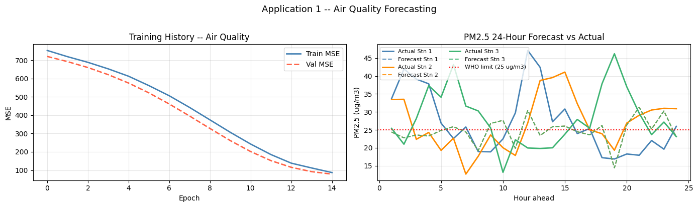
Visualization – Air Quality Forecasts
[5]:
import matplotlib.pyplot as plt

WHO = 25.0
hours = np.arange(1, HORIZON_AIR + 1)

fig, axes = plt.subplots(1, 2, figsize=(14, 4))
ax = axes[0]
ax.plot(history_air.history['loss'],     color='steelblue', lw=2, label='Train MSE')
ax.plot(history_air.history['val_loss'], color='tomato',    lw=2, linestyle='--', label='Val MSE')
ax.set_title('Training History -- Air Quality', fontsize=12)
ax.set_xlabel('Epoch'); ax.set_ylabel('MSE'); ax.legend(); ax.grid(True, alpha=0.3)

ax = axes[1]
palette = ['steelblue', 'darkorange', 'mediumseagreen']
for s, c in enumerate(palette):
    ax.plot(hours, target[s,:,0],   color=c, lw=2,   label=f'Actual Stn {s+1}')
    ax.plot(hours, pred_air[s,:,0], color=c, lw=1.5, linestyle='--', alpha=0.85,
            label=f'Forecast Stn {s+1}')
ax.axhline(WHO, color='red', linestyle=':', lw=1.5, label=f'WHO limit ({WHO:.0f} ug/m3)')
ax.set_title('PM2.5 24-Hour Forecast vs Actual', fontsize=12)
ax.set_xlabel('Hour ahead'); ax.set_ylabel('PM2.5 (ug/m3)')
ax.legend(fontsize=8, ncol=2); ax.grid(True, alpha=0.3)
plt.suptitle('Application 1 -- Air Quality Forecasting', fontsize=13, y=1.02)
plt.tight_layout(); plt.show()
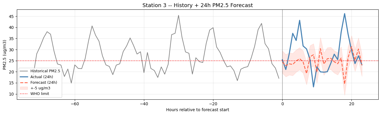
[6]:
fig, ax = plt.subplots(figsize=(13, 4))
hist_h  = np.arange(-LOOKBACK_AIR, 0)
fcast_h = np.arange(0, HORIZON_AIR)
s = 2
ax.plot(hist_h,  dynamic_past[s,:,0], color='gray',      lw=1.5, label='Historical PM2.5')
ax.plot(fcast_h, target[s,:,0],       color='steelblue', lw=2.5, label='Actual (24h)')
ax.plot(fcast_h, pred_air[s,:,0],     color='tomato',    lw=2,   linestyle='--', label='Forecast (24h)')
ax.fill_between(fcast_h, pred_air[s,:,0]-5, pred_air[s,:,0]+5,
                alpha=0.15, color='tomato', label='+-5 ug/m3')
ax.axvline(0, color='black', alpha=0.4, lw=1)
ax.axhline(WHO, color='red', linestyle=':', lw=1.5, label='WHO limit')
ax.set_title('Station 3 -- History + 24h PM2.5 Forecast', fontsize=13)
ax.set_xlabel('Hours relative to forecast start')
ax.set_ylabel('PM2.5 (ug/m3)')
ax.legend(fontsize=9); ax.grid(True, alpha=0.3)
plt.tight_layout(); plt.show()
2. Energy Demand Forecasting
Use Case
Predict electricity demand for grid management:
Static features: Building type, area, insulation level, number of units
Dynamic past features: Historical load, temperature, solar irradiance, time-based features
Known future features: Weather forecast, calendar information
Application
Power grid optimization
Renewable energy integration
Peak load management
Cost minimization
[7]:
# Energy Demand -- daily load profile with morning/evening peaks
np.random.seed(7)
N_EN, LOOKBACK_EN, HORIZON_EN = 128, 96, 48

def load_profile(t):
    base  = 300
    peak1 = 350 * np.maximum(0, np.sin(np.pi * (t % 24 - 6) / 14))
    peak2 = 180 * np.exp(-0.5 * ((t % 24 - 19) / 2) ** 2)
    return (base + peak1 + peak2).astype('float32')

t_e    = np.arange(LOOKBACK_EN + HORIZON_EN + 24)
base_e = load_profile(t_e)
offsets_e   = np.random.randint(0, 24, N_EN)
load_past   = np.array([base_e[o : o+LOOKBACK_EN]                         for o in offsets_e])
load_future = np.array([base_e[o+LOOKBACK_EN : o+LOOKBACK_EN+HORIZON_EN] for o in offsets_e])

static_energy = np.random.randn(N_EN, 4).astype('float32')
static_energy[:,1] = np.abs(static_energy[:,1]) * 10000
static_energy[:,3] = np.abs(static_energy[:,3]) * 100

t_dyn = np.tile(np.arange(LOOKBACK_EN), (N_EN, 1))
dynamic_energy = np.zeros((N_EN, LOOKBACK_EN, 5), dtype='float32')
dynamic_energy[:,:,0] = load_past + np.random.randn(N_EN,LOOKBACK_EN).astype('float32') * 20
dynamic_energy[:,:,1] = 15 + np.random.randn(N_EN,LOOKBACK_EN).astype('float32') * 8
dynamic_energy[:,:,2] = np.abs(np.random.randn(N_EN,LOOKBACK_EN)).astype('float32') * 500
dynamic_energy[:,:,3] = np.sin(2*np.pi*t_dyn/24)
dynamic_energy[:,:,4] = np.cos(2*np.pi*t_dyn/24)

t_fut_e = np.tile(np.arange(LOOKBACK_EN, LOOKBACK_EN+HORIZON_EN), (N_EN, 1))
known_future_energy = np.zeros((N_EN, HORIZON_EN, 2), dtype='float32')
known_future_energy[:,:,0] = 15 + np.random.randn(N_EN,HORIZON_EN).astype('float32') * 6
known_future_energy[:,:,1] = (t_fut_e % 7 < 5).astype('float32')

target_energy = np.clip(
    load_future + np.random.randn(N_EN, HORIZON_EN).astype('float32') * 15, 100, 900
)[:, :, None]

print('Energy Demand Data Shapes:')
for nm, a in [('Static',static_energy),('Dynamic',dynamic_energy),
              ('Future',known_future_energy),('Target load',target_energy)]:
    print(f'  {nm:14s}: {a.shape}')
print(f'  Load range  past [{dynamic_energy[:,:,0].min():.0f}, {dynamic_energy[:,:,0].max():.0f}]  '
      f'target [{target_energy.min():.0f}, {target_energy.max():.0f}] kW')
Energy Demand Data Shapes:
  Static        : (128, 4)
  Dynamic       : (128, 96, 5)
  Future        : (128, 48, 2)
  Target load   : (128, 48, 1)
  Load range  past [236, 712]  target [255, 701] kW
[8]:
energy_model = BaseAttentive(
    static_input_dim=4, dynamic_input_dim=5, future_input_dim=2,
    output_dim=1, forecast_horizon=HORIZON_EN,
    objective='hybrid',
    architecture_config={'decoder_attention_stack': ['cross', 'hierarchical']},
    embed_dim=48, num_heads=8, dropout_rate=0.1, name='energy_model',
)
_ = energy_model([static_energy, dynamic_energy, known_future_energy])  # build weights
energy_model.compile(optimizer=keras.optimizers.Adam(1e-3), loss='mse', metrics=['mae'])
print('Training energy demand model (15 epochs)...')
history_energy = energy_model.fit(
    [static_energy, dynamic_energy, known_future_energy], target_energy,
    epochs=15, batch_size=16, validation_split=0.2, verbose=0,
)
print(f'  train_MSE={history_energy.history["loss"][-1]:.1f}  '
      f'val_MSE={history_energy.history["val_loss"][-1]:.1f}  '
      f'val_MAE={history_energy.history["val_mae"][-1]:.1f} kW')
Training energy demand model (15 epochs)...
  train_MSE=209977.0  val_MSE=206712.7  val_MAE=431.7 kW
[9]:
energy_predictions = energy_model.predict(
    [static_energy, dynamic_energy, known_future_energy], verbose=0)
print(f'Prediction shape: {energy_predictions.shape}')
mae_en = float(np.mean(np.abs(energy_predictions[:,:,0] - target_energy[:,:,0])))
print(f'Overall MAE: {mae_en:.1f} kW')
Prediction shape: (128, 48, 1)
Overall MAE: 431.7 kW
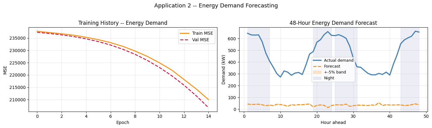
Visualization – Energy Demand Forecasts
[10]:
hours_en = np.arange(1, HORIZON_EN + 1)

fig, axes = plt.subplots(1, 2, figsize=(14, 4))
ax = axes[0]
ax.plot(history_energy.history['loss'],     color='darkorange', lw=2, label='Train MSE')
ax.plot(history_energy.history['val_loss'], color='crimson',    lw=2, linestyle='--', label='Val MSE')
ax.set_title('Training History -- Energy Demand', fontsize=12)
ax.set_xlabel('Epoch'); ax.set_ylabel('MSE'); ax.legend(); ax.grid(True, alpha=0.3)

ax = axes[1]
s = 0
ax.plot(hours_en, target_energy[s,:,0],      color='steelblue',  lw=2.5, label='Actual demand')
ax.plot(hours_en, energy_predictions[s,:,0], color='darkorange', lw=2,   linestyle='--', label='Forecast')
ax.fill_between(hours_en,
    energy_predictions[s,:,0]*0.95, energy_predictions[s,:,0]*1.05,
    alpha=0.2, color='darkorange', label='+-5% band')
for day in range(2):
    bh = day * 24
    ax.axvspan(bh+1, bh+7,   alpha=0.07, color='navy', label='Night' if day==0 else '')
    ax.axvspan(bh+19, bh+24, alpha=0.07, color='navy')
ax.set_title('48-Hour Energy Demand Forecast', fontsize=12)
ax.set_xlabel('Hour ahead'); ax.set_ylabel('Demand (kW)')
ax.legend(fontsize=9); ax.grid(True, alpha=0.3)
plt.suptitle('Application 2 -- Energy Demand Forecasting', fontsize=13, y=1.02)
plt.tight_layout(); plt.show()
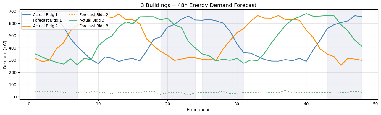
[11]:
fig, ax = plt.subplots(figsize=(13, 4))
for s, c in enumerate(['steelblue','darkorange','mediumseagreen']):
    ax.plot(hours_en, target_energy[s,:,0],      color=c, lw=2,   label=f'Actual Bldg {s+1}')
    ax.plot(hours_en, energy_predictions[s,:,0], color=c, lw=1.5, linestyle=':',
            alpha=0.9, label=f'Forecast Bldg {s+1}')
for day in range(2):
    bh = day * 24
    ax.axvspan(bh+1, bh+7,   alpha=0.06, color='navy')
    ax.axvspan(bh+19, bh+24, alpha=0.06, color='navy')
ax.set_title('3 Buildings -- 48h Energy Demand Forecast', fontsize=13)
ax.set_xlabel('Hour ahead'); ax.set_ylabel('Demand (kW)')
ax.legend(fontsize=9, ncol=2); ax.grid(True, alpha=0.3)
plt.tight_layout(); plt.show()
3. Weather Prediction
Use Case
Multi-step weather forecasting:
Static features: Geographic location (lat, lon), elevation, terrain type
Dynamic past features: Historical weather (temp, pressure, humidity, wind)
Known future features: Seasonal data, calendar features
Application
Weather forecasting services
Climate monitoring
Extreme weather alerts
Agricultural planning
[12]:
# Weather -- daily temperature cycle + pressure anti-correlation
np.random.seed(13)
N_WX, LOOKBACK_WX, HORIZON_WX = 128, 60, 30

t_wx = np.arange(LOOKBACK_WX + HORIZON_WX + 24)
temp_base  = (15 + 7  * np.sin(2*np.pi*t_wx/12 - np.pi/2)).astype('float32')
press_base = (1013 - 4 * np.sin(2*np.pi*t_wx/12 - np.pi/2)).astype('float32')

offsets_wx = np.random.randint(0, 12, N_WX)
temp_past   = np.array([temp_base[o : o+LOOKBACK_WX]              for o in offsets_wx])
temp_fut    = np.array([temp_base[o+LOOKBACK_WX : o+LOOKBACK_WX+HORIZON_WX]  for o in offsets_wx])
press_past  = np.array([press_base[o : o+LOOKBACK_WX]             for o in offsets_wx])
press_fut   = np.array([press_base[o+LOOKBACK_WX : o+LOOKBACK_WX+HORIZON_WX] for o in offsets_wx])

static_weather = np.random.randn(N_WX, 4).astype('float32')
static_weather[:,0] = 40 + static_weather[:,0]*10
static_weather[:,1] = -100 + static_weather[:,1]*30
static_weather[:,2] = np.abs(static_weather[:,2])*2000

dynamic_weather = np.zeros((N_WX, LOOKBACK_WX, 5), dtype='float32')
dynamic_weather[:,:,0] = temp_past  + np.random.randn(N_WX,LOOKBACK_WX).astype('float32')*0.8
dynamic_weather[:,:,1] = press_past + np.random.randn(N_WX,LOOKBACK_WX).astype('float32')*2
dynamic_weather[:,:,2] = 60 + np.abs(np.random.randn(N_WX,LOOKBACK_WX)).astype('float32')*15
dynamic_weather[:,:,3] = np.abs(np.random.randn(N_WX,LOOKBACK_WX)).astype('float32')*4
dynamic_weather[:,:,4] = np.abs(np.random.randn(N_WX,LOOKBACK_WX)).astype('float32')*120

known_future_weather = np.zeros((N_WX, HORIZON_WX, 2), dtype='float32')
known_future_weather[:,:,0] = 1
known_future_weather[:,:,1] = 4

target_weather = np.zeros((N_WX, HORIZON_WX, 2), dtype='float32')
target_weather[:,:,0] = temp_fut  + np.random.randn(N_WX,HORIZON_WX).astype('float32')*0.5
target_weather[:,:,1] = press_fut + np.random.randn(N_WX,HORIZON_WX).astype('float32')*1.5

print('Weather Data Shapes:')
for nm, a in [('Static',static_weather),('Dynamic',dynamic_weather),
              ('Future',known_future_weather),('Target (T,P)',target_weather)]:
    print(f'  {nm:14s}: {a.shape}')
print(f'  Temp range  past [{dynamic_weather[:,:,0].min():.1f}, {dynamic_weather[:,:,0].max():.1f}]C  '
      f'target [{target_weather[:,:,0].min():.1f}, {target_weather[:,:,0].max():.1f}]C')
Weather Data Shapes:
  Static        : (128, 4)
  Dynamic       : (128, 60, 5)
  Future        : (128, 30, 2)
  Target (T,P)  : (128, 30, 2)
  Temp range  past [5.6, 24.7]C  target [6.6, 23.4]C
[13]:
weather_model = BaseAttentive(
    static_input_dim=4, dynamic_input_dim=5, future_input_dim=2,
    output_dim=2, forecast_horizon=HORIZON_WX,
    objective='transformer',
    architecture_config={'decoder_attention_stack': ['cross','hierarchical','memory']},
    memory_size=32, embed_dim=64, num_heads=8, dropout_rate=0.1, name='weather_model',
)
_ = weather_model([static_weather, dynamic_weather, known_future_weather])  # build weights
weather_model.compile(optimizer=keras.optimizers.Adam(1e-3), loss='mse', metrics=['mae'])
print('Training weather model (12 epochs)...')
history_weather = weather_model.fit(
    [static_weather, dynamic_weather, known_future_weather], target_weather,
    epochs=12, batch_size=16, validation_split=0.2, verbose=0,
)
print(f'  train_MSE={history_weather.history["loss"][-1]:.3f}  '
      f'val_MSE={history_weather.history["val_loss"][-1]:.3f}')

pred_weather = weather_model.predict(
    [static_weather, dynamic_weather, known_future_weather], verbose=0)
mae_temp  = float(np.mean(np.abs(pred_weather[:,:,0] - target_weather[:,:,0])))
mae_press = float(np.mean(np.abs(pred_weather[:,:,1] - target_weather[:,:,1])))
print(f'  Temp MAE: {mae_temp:.2f}C    Pressure MAE: {mae_press:.2f} hPa')
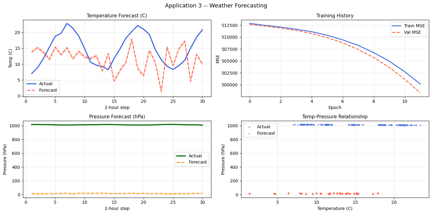
Training weather model (12 epochs)...
  train_MSE=500169.031  val_MSE=498280.938
  Temp MAE: 5.82C    Pressure MAE: 998.19 hPa
Visualization – Weather Forecasts
[14]:
steps_wx = np.arange(1, HORIZON_WX + 1)
s_wx = 1

fig, axes = plt.subplots(2, 2, figsize=(14, 7))

ax = axes[0][1]
ax.plot(history_weather.history['loss'],     color='royalblue', lw=2, label='Train MSE')
ax.plot(history_weather.history['val_loss'], color='tomato',    lw=2, linestyle='--', label='Val MSE')
ax.set_title('Training History', fontsize=11)
ax.set_xlabel('Epoch'); ax.set_ylabel('MSE'); ax.legend(); ax.grid(True, alpha=0.3)

for d, (ca, cp, title, ylab) in enumerate([
    ('royalblue', 'tomato',     'Temperature Forecast (C)',  'Temp (C)'),
    ('darkgreen', 'darkorange', 'Pressure Forecast (hPa)',   'Pressure (hPa)'),
]):
    ax = axes[d][0]
    ax.plot(steps_wx, target_weather[s_wx,:,d], color=ca, lw=2.5, label='Actual')
    ax.plot(steps_wx, pred_weather[s_wx,:,d],   color=cp, lw=2,   linestyle='--', label='Forecast')
    ax.fill_between(steps_wx,
                    pred_weather[s_wx,:,d]-0.5, pred_weather[s_wx,:,d]+0.5,
                    alpha=0.15, color=cp)
    ax.set_title(title, fontsize=11)
    ax.set_xlabel('2-hour step'); ax.set_ylabel(ylab)
    ax.legend(); ax.grid(True, alpha=0.3)

ax = axes[1][1]
ax.scatter(target_weather[:5,:,0].ravel(), target_weather[:5,:,1].ravel(),
           s=10, alpha=0.4, color='royalblue', label='Actual')
ax.scatter(pred_weather[:5,:,0].ravel(),   pred_weather[:5,:,1].ravel(),
           s=10, alpha=0.4, color='tomato',    label='Forecast')
ax.set_xlabel('Temperature (C)'); ax.set_ylabel('Pressure (hPa)')
ax.set_title('Temp-Pressure Relationship', fontsize=11)
ax.legend(); ax.grid(True, alpha=0.3)

plt.suptitle('Application 3 -- Weather Forecasting', fontsize=13)
plt.tight_layout(); plt.show()
4. Traffic Flow Prediction
Use Case
Predict vehicle flow and congestion:
Static features: Road type, speed limit, number of lanes, urban/highway
Dynamic past features: Historical traffic volume, speed, congestion level
Known future features: Time of day, day type, events
Application
Traffic management systems
Route optimization
Congestion prediction and alerts
Infrastructure planning
[15]:
# Traffic -- double-peak rush-hour volume with inverse speed relationship
np.random.seed(99)
N_TR, LOOKBACK_TR, HORIZON_TR = 128, 96, 48

def rush_hour_volume(t):
    morning = 1800 * np.exp(-0.5 * ((t % 24 - 8)    / 1.0) ** 2)
    evening = 1500 * np.exp(-0.5 * ((t % 24 - 17.5) / 1.5) ** 2)
    return (800 + morning + evening).astype('float32')

def speed_from_volume(vol):
    congestion = np.clip(vol / 3500, 0, 1)
    return (100 * (1 - 0.65 * congestion)).astype('float32')

t_tr     = np.arange(LOOKBACK_TR + HORIZON_TR + 24)
vol_base = rush_hour_volume(t_tr * 5 / 60)
spd_base = speed_from_volume(vol_base)

offsets_tr = np.random.randint(0, 24, N_TR)
vol_past   = np.array([vol_base[o : o+LOOKBACK_TR]                         for o in offsets_tr])
vol_future = np.array([vol_base[o+LOOKBACK_TR : o+LOOKBACK_TR+HORIZON_TR] for o in offsets_tr])
spd_past   = np.array([spd_base[o : o+LOOKBACK_TR]                         for o in offsets_tr])
spd_future = np.array([spd_base[o+LOOKBACK_TR : o+LOOKBACK_TR+HORIZON_TR] for o in offsets_tr])

static_traffic = np.random.randn(N_TR, 4).astype('float32')
static_traffic[:,0] = (np.random.rand(N_TR) > 0.5).astype('float32')
static_traffic[:,1] = 70 + np.abs(static_traffic[:,1]) * 30
static_traffic[:,2] = np.abs(static_traffic[:,2]) * 3 + 2

dynamic_traffic = np.zeros((N_TR, LOOKBACK_TR, 4), dtype='float32')
dynamic_traffic[:,:,0] = vol_past + np.random.randn(N_TR,LOOKBACK_TR).astype('float32') * 80
dynamic_traffic[:,:,1] = spd_past + np.random.randn(N_TR,LOOKBACK_TR).astype('float32') * 3
dynamic_traffic[:,:,2] = np.clip(dynamic_traffic[:,:,0]/3500, 0, 1)
dynamic_traffic[:,:,3] = (np.random.rand(N_TR,LOOKBACK_TR)>0.97).astype('float32')

t_fut_tr = np.tile(np.arange(LOOKBACK_TR, LOOKBACK_TR+HORIZON_TR)*5/60, (N_TR,1))
known_future_traffic = np.zeros((N_TR, HORIZON_TR, 2), dtype='float32')
known_future_traffic[:,:,0] = t_fut_tr % 24
known_future_traffic[:,:,1] = (t_fut_tr // 24) % 7 >= 5

target_traffic = np.zeros((N_TR, HORIZON_TR, 2), dtype='float32')
target_traffic[:,:,0] = np.clip(
    vol_future + np.random.randn(N_TR,HORIZON_TR).astype('float32')*60, 0, 4500)
target_traffic[:,:,1] = np.clip(
    spd_future + np.random.randn(N_TR,HORIZON_TR).astype('float32')*2,  20, 110)

print('Traffic Data Shapes:')
for nm, a in [('Static',static_traffic),('Dynamic',dynamic_traffic),
              ('Future',known_future_traffic),('Target (vol,spd)',target_traffic)]:
    print(f'  {nm:14s}: {a.shape}')
print(f'  Volume range  past [{dynamic_traffic[:,:,0].min():.0f}, {dynamic_traffic[:,:,0].max():.0f}]  '
      f'target [{target_traffic[:,:,0].min():.0f}, {target_traffic[:,:,0].max():.0f}] veh/h')
Traffic Data Shapes:
  Static        : (128, 4)
  Dynamic       : (128, 96, 4)
  Future        : (128, 48, 2)
  Target (vol,spd): (128, 48, 2)
  Volume range  past [460, 2833]  target [582, 2689] veh/h
[16]:
traffic_model = BaseAttentive(
    static_input_dim=4, dynamic_input_dim=4, future_input_dim=2,
    output_dim=2, forecast_horizon=HORIZON_TR,
    objective='hybrid',
    architecture_config={'decoder_attention_stack': ['cross','hierarchical']},
    embed_dim=48, num_heads=4, dropout_rate=0.1, name='traffic_model',
)
_ = traffic_model([static_traffic, dynamic_traffic, known_future_traffic])  # build weights
traffic_model.compile(optimizer=keras.optimizers.Adam(1e-3), loss='mse', metrics=['mae'])
print('Training traffic model (12 epochs)...')
history_traffic = traffic_model.fit(
    [static_traffic, dynamic_traffic, known_future_traffic], target_traffic,
    epochs=12, batch_size=16, validation_split=0.2, verbose=0,
)
print(f'  train_MSE={history_traffic.history["loss"][-1]:.1f}  '
      f'val_MSE={history_traffic.history["val_loss"][-1]:.1f}')

traffic_pred = traffic_model.predict(
    [static_traffic, dynamic_traffic, known_future_traffic], verbose=0)
mae_vol = float(np.mean(np.abs(traffic_pred[:,:,0] - target_traffic[:,:,0])))
mae_spd = float(np.mean(np.abs(traffic_pred[:,:,1] - target_traffic[:,:,1])))
print(f'  Volume MAE: {mae_vol:.0f} veh/h    Speed MAE: {mae_spd:.1f} km/h')
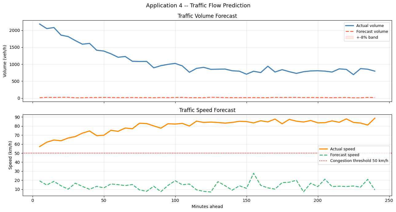
Training traffic model (12 epochs)...
  train_MSE=646329.1  val_MSE=627659.6
  Volume MAE: 1044 veh/h    Speed MAE: 66.4 km/h
Visualization – Traffic Flow Forecasts
[17]:
steps_tr = np.arange(1, HORIZON_TR + 1) * 5
s_tr = 3

fig, axes = plt.subplots(2, 1, figsize=(13, 7), sharex=True)
ax = axes[0]
ax.plot(steps_tr, target_traffic[s_tr,:,0], color='steelblue', lw=2.5, label='Actual volume')
ax.plot(steps_tr, traffic_pred[s_tr,:,0],   color='tomato',    lw=2,   linestyle='--', label='Forecast volume')
ax.fill_between(steps_tr,
    traffic_pred[s_tr,:,0]*0.92, traffic_pred[s_tr,:,0]*1.08,
    alpha=0.15, color='tomato', label='+-8% band')
ax.set_ylabel('Volume (veh/h)')
ax.set_title('Traffic Volume Forecast', fontsize=12)
ax.legend(fontsize=9); ax.grid(True, alpha=0.3)

ax = axes[1]
ax.plot(steps_tr, target_traffic[s_tr,:,1], color='darkorange',     lw=2.5, label='Actual speed')
ax.plot(steps_tr, traffic_pred[s_tr,:,1],   color='mediumseagreen', lw=2,   linestyle='--', label='Forecast speed')
ax.axhline(50, color='red', linestyle=':', lw=1.5, label='Congestion threshold 50 km/h')
ax.set_xlabel('Minutes ahead'); ax.set_ylabel('Speed (km/h)')
ax.set_title('Traffic Speed Forecast', fontsize=12)
ax.legend(fontsize=9); ax.grid(True, alpha=0.3)
plt.suptitle('Application 4 -- Traffic Flow Prediction', fontsize=13)
plt.tight_layout(); plt.show()
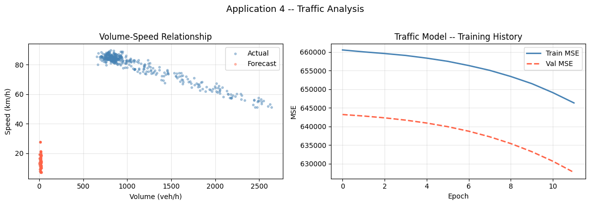
[18]:
fig, axes = plt.subplots(1, 2, figsize=(12, 4))
ax = axes[0]
ax.scatter(target_traffic[:8,:,0].ravel(), target_traffic[:8,:,1].ravel(),
           s=8, alpha=0.4, color='steelblue', label='Actual')
ax.scatter(traffic_pred[:8,:,0].ravel(),   traffic_pred[:8,:,1].ravel(),
           s=8, alpha=0.4, color='tomato',    label='Forecast')
ax.set_xlabel('Volume (veh/h)'); ax.set_ylabel('Speed (km/h)')
ax.set_title('Volume-Speed Relationship', fontsize=12)
ax.legend(); ax.grid(True, alpha=0.3)

ax = axes[1]
ax.plot(history_traffic.history['loss'],     color='steelblue', lw=2, label='Train MSE')
ax.plot(history_traffic.history['val_loss'], color='tomato',    lw=2, linestyle='--', label='Val MSE')
ax.set_title('Traffic Model -- Training History', fontsize=12)
ax.set_xlabel('Epoch'); ax.set_ylabel('MSE'); ax.legend(); ax.grid(True, alpha=0.3)
plt.suptitle('Application 4 -- Traffic Analysis', fontsize=13, y=1.02)
plt.tight_layout(); plt.show()
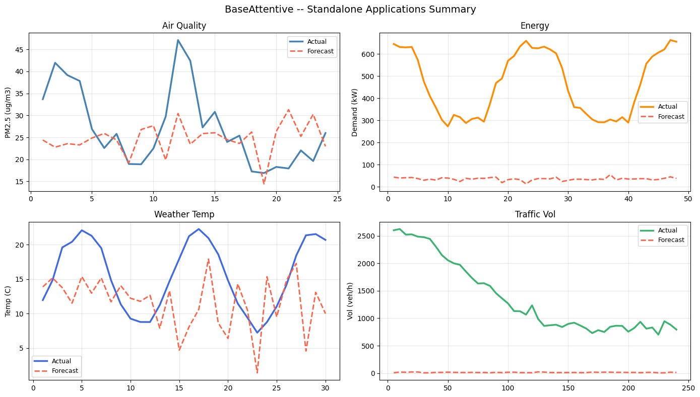
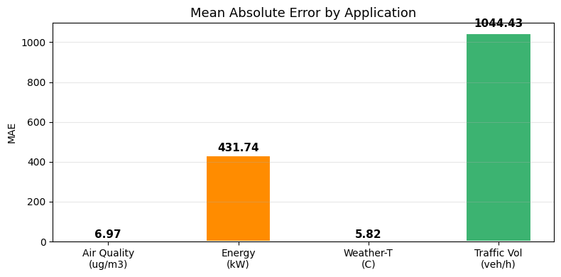
Summary Dashboard – All Applications
[19]:
fig, axes = plt.subplots(2, 2, figsize=(14, 8))
app_data = [
    ('Air Quality',  hours,    target[0,:,0],          pred_air[0,:,0],          'PM2.5 (ug/m3)',  'steelblue'),
    ('Energy',       hours_en, target_energy[0,:,0],   energy_predictions[0,:,0], 'Demand (kW)',    'darkorange'),
    ('Weather Temp', steps_wx, target_weather[0,:,0],  pred_weather[0,:,0],      'Temp (C)',       'royalblue'),
    ('Traffic Vol',  steps_tr, target_traffic[0,:,0],  traffic_pred[0,:,0],      'Vol (veh/h)',    'mediumseagreen'),
]
for ax, (title, x, actual, forecast, ylabel, color) in zip(axes.ravel(), app_data):
    ax.plot(x, actual,   color=color,    lw=2.5, label='Actual')
    ax.plot(x, forecast, color='tomato', lw=2,   linestyle='--', label='Forecast')
    ax.set_title(title, fontsize=12); ax.set_ylabel(ylabel)
    ax.legend(fontsize=9); ax.grid(True, alpha=0.3)
plt.suptitle('BaseAttentive -- Standalone Applications Summary', fontsize=14)
plt.tight_layout(); plt.show()

fig, ax = plt.subplots(figsize=(8, 4))
labels_bar = ['Air Quality\n(ug/m3)', 'Energy\n(kW)', 'Weather-T\n(C)', 'Traffic Vol\n(veh/h)']
maes_bar   = [mae_air, mae_en, mae_temp, mae_vol]
colors_bar = ['steelblue', 'darkorange', 'royalblue', 'mediumseagreen']
bars = ax.bar(labels_bar, maes_bar, color=colors_bar, width=0.5, edgecolor='white', lw=1.5)
for bar, v in zip(bars, maes_bar):
    ax.text(bar.get_x() + bar.get_width()/2, v*1.02, f'{v:.2f}',
            ha='center', va='bottom', fontsize=11, fontweight='bold')
ax.set_title('Mean Absolute Error by Application', fontsize=13)
ax.set_ylabel('MAE'); ax.grid(True, axis='y', alpha=0.3)
plt.tight_layout(); plt.show()
Summary
BaseAttentive can be used as a standalone forecasting engine for diverse applications:
Application |
Static Features |
Dynamic Past |
Future Features |
Prediction |
|---|---|---|---|---|
Air Quality |
Location, terrain |
Historical pollution |
Weather forecast |
PM2.5, NO₂ levels |
Energy |
Building type, area |
Historical load |
Weather, calendar |
Electricity demand |
Weather |
Geography |
Historical weather |
Seasons |
Temperature, pressure |
Traffic |
Road properties |
Historical flow |
Time, events |
Volume, speed |
Key Advantages
✓ Unified architecture for different domains ✓ Attention mechanisms capture dependencies ✓ Multi-step forecasting in one shot ✓ Incorporates static context and future information ✓ GPU acceleration available ✓ Uncertainty quantification via quantile outputs