BaseAttentive as a Kernel for Robust Neural Networks
This notebook demonstrates using BaseAttentive as a kernel component within larger neural network architectures for building robust, production-ready forecasting systems.
Table of Contents
Ensemble Methods with Multiple BaseAttentive Models
Physics-Guided Neural Networks with BaseAttentive
Transfer Learning and Domain Adaptation
Multi-Task Learning for Correlated Predictions
Setup and Imports
[1]:
import os
import warnings

import numpy as np

warnings.filterwarnings("ignore")

# ── v2.2.0 Backend Setup ─────────────────────────────────────────────────────
# BASE_ATTENTIVE_BACKEND must be set *before* importing base_attentive.
# Choose your installed backend: "tensorflow" | "torch" | "jax" | "auto"
os.environ.setdefault("BASE_ATTENTIVE_BACKEND", "tensorflow")
os.environ.setdefault("KERAS_BACKEND", os.environ["BASE_ATTENTIVE_BACKEND"])
BACKEND = os.environ["BASE_ATTENTIVE_BACKEND"]

import keras

from base_attentive import BaseAttentive, __version__

print(f"BaseAttentive {__version__} — backend: {BACKEND}")
BaseAttentive 2.2.0 — backend: tensorflow
1. Ensemble Methods: Robust Predictions via BaseAttentive Kernels
Concept
Combine multiple BaseAttentive models with different architectures to reduce overfitting and improve robustness:
Model 1: Hybrid (attention + LSTM)
Model 2: Pure transformer (self-attention only)
Model 3: LSTM-heavy (attention heads tuned to past)
Architecture
Inputs (static, dynamic_past, future)
    ↓
BaseAttentive Kernel 1 → predictions_1
    ↓ (parallel)
BaseAttentive Kernel 2 → predictions_2
    ↓ (parallel)
BaseAttentive Kernel 3 → predictions_3
    ↓
Ensemble Layer (weighted average or meta-learner)
    ↓
Final Predictions (robust)
[2]:
# Structured sine-wave data for ensemble demonstration
import numpy as np
np.random.seed(42)
batch_size = 64
LOOKBACK, HORIZON = 48, 24

# Structured pattern: sine wave + harmonic
t_past   = np.linspace(0, 4*np.pi, LOOKBACK)
t_future = np.linspace(4*np.pi, 6*np.pi, HORIZON)

static_features = np.random.randn(batch_size, 4).astype('float32')
dynamic_past = (np.tile(np.sin(t_past), (batch_size,1))[:,:,None]
                + 0.3*np.sin(2*t_past)[None,:,None]
                + 0.1*np.random.randn(batch_size,LOOKBACK,5)).astype('float32')[:,:,:5]
# Fix: broadcast properly
dynamic_past = np.zeros((batch_size, LOOKBACK, 5), dtype='float32')
for d in range(5):
    dynamic_past[:,:,d] = (np.tile(np.sin(t_past*(1+d*0.1)), (batch_size,1))
                           + 0.1*np.random.randn(batch_size,LOOKBACK))

known_future = np.zeros((batch_size, HORIZON, 2), dtype='float32')
for d in range(2):
    known_future[:,:,d] = (np.tile(np.cos(t_future*(1+d*0.2)), (batch_size,1))
                           + 0.1*np.random.randn(batch_size,HORIZON))

target = (np.tile(np.sin(t_future), (batch_size,1))[:,:,None]
          + 0.1*np.random.randn(batch_size,HORIZON,1)).astype('float32')

print(f'Ensemble data -- static:{static_features.shape}  '
      f'dynamic:{dynamic_past.shape}  future:{known_future.shape}  target:{target.shape}')
Ensemble data -- static:(64, 4) dynamic:(64, 48, 5) future:(64, 24, 2) target:(64, 24, 1)
[3]:
# Create 3 individual BaseAttentive kernels
kernel_1 = BaseAttentive(
    static_input_dim=4, dynamic_input_dim=5, future_input_dim=2,
    forecast_horizon=HORIZON, objective='hybrid',
    architecture_config={'decoder_attention_stack': ['cross', 'hierarchical']},
    embed_dim=32, num_heads=4, name='kernel_hybrid',
)
kernel_2 = BaseAttentive(
    static_input_dim=4, dynamic_input_dim=5, future_input_dim=2,
    forecast_horizon=HORIZON, objective='transformer',
    architecture_config={'decoder_attention_stack': ['cross', 'hierarchical']},
    embed_dim=32, num_heads=4, name='kernel_transformer',
)
kernel_3 = BaseAttentive(
    static_input_dim=4, dynamic_input_dim=5, future_input_dim=2,
    forecast_horizon=HORIZON, objective='hybrid',
    architecture_config={'decoder_attention_stack': ['memory', 'cross']},
    memory_size=32, embed_dim=32, num_heads=4, name='kernel_memory',
)
print('Created 3 BaseAttentive kernels for ensemble')
Created 3 BaseAttentive kernels for ensemble
[4]:
# Build kernels with concrete data before using in functional API
_ = kernel_1([static_features, dynamic_past, known_future])
_ = kernel_2([static_features, dynamic_past, known_future])
_ = kernel_3([static_features, dynamic_past, known_future])

# Build ensemble model using Keras functional API
static_input  = keras.Input(shape=(4,),          name='static')
dynamic_input = keras.Input(shape=(LOOKBACK, 5), name='dynamic_past')
future_input  = keras.Input(shape=(HORIZON, 2),  name='known_future')

pred_1 = kernel_1([static_input, dynamic_input, future_input])
pred_2 = kernel_2([static_input, dynamic_input, future_input])
pred_3 = kernel_3([static_input, dynamic_input, future_input])

ensemble_concat   = keras.layers.Concatenate(axis=-1)([pred_1, pred_2, pred_3])
ensemble_combined = keras.layers.Dense(16, activation='relu')(ensemble_concat)
ensemble_output   = keras.layers.Dense(1)(ensemble_combined)  # shape: (batch, HORIZON, 1)

ensemble_model = keras.Model(
    inputs=[static_input, dynamic_input, future_input],
    outputs=ensemble_output,
    name='BaseAttentive_Ensemble',
)
ensemble_model.compile(optimizer=keras.optimizers.Adam(1e-3), loss='mse', metrics=['mae'])
print('Ensemble model built.')
Ensemble model built.
[5]:
print('Training ensemble model (15 epochs)...')
history_ensemble = ensemble_model.fit(
    [static_features, dynamic_past, known_future], target,
    epochs=15, batch_size=16, validation_split=0.2, verbose=0,
)

# Get predictions from individual kernels + ensemble
pred_k1 = kernel_1.predict([static_features, dynamic_past, known_future], verbose=0)
pred_k2 = kernel_2.predict([static_features, dynamic_past, known_future], verbose=0)
pred_k3 = kernel_3.predict([static_features, dynamic_past, known_future], verbose=0)
ensemble_predictions = ensemble_model.predict(
    [static_features, dynamic_past, known_future], verbose=0)

print(f'Ensemble MSE={history_ensemble.history["loss"][-1]:.4f}  '
      f'val={history_ensemble.history["val_loss"][-1]:.4f}')
print(f'Prediction shape: {ensemble_predictions.shape}')
Training ensemble model (15 epochs)...
Ensemble MSE=0.0303  val=0.0124
Prediction shape: (64, 24, 1)
Visualization – Ensemble Architecture
[6]:
import matplotlib.pyplot as plt

steps = np.arange(1, HORIZON + 1)
s = 0

fig, axes = plt.subplots(1, 2, figsize=(14, 4))

# Left: individual kernels + ensemble + actual
ax = axes[0]
ax.plot(steps, target[s,:,0],               color='black',       lw=2.5,  label='Actual',          zorder=5)
ax.plot(steps, pred_k1[s,:,0],              color='steelblue',   lw=1.2,  label='Kernel 1 (Hybrid)',   alpha=0.7)
ax.plot(steps, pred_k2[s,:,0],              color='darkorange',  lw=1.2,  label='Kernel 2 (Transformer)', alpha=0.7)
ax.plot(steps, pred_k3[s,:,0],              color='mediumseagreen', lw=1.2, label='Kernel 3 (Memory)', alpha=0.7)
ax.plot(steps, ensemble_predictions[s,:,0], color='crimson',     lw=2.5,  label='Ensemble',         zorder=4)
# Uncertainty band: std across kernels
stack = np.stack([pred_k1[:,:,0], pred_k2[:,:,0], pred_k3[:,:,0]], axis=0)
band_lo = stack.min(axis=0)[s]
band_hi = stack.max(axis=0)[s]
ax.fill_between(steps, band_lo, band_hi, alpha=0.15, color='crimson', label='Kernel range')
ax.set_title('Ensemble vs Individual Kernels', fontsize=12)
ax.set_xlabel('Forecast step'); ax.set_ylabel('Value')
ax.legend(fontsize=8); ax.grid(True, alpha=0.3)

# Right: training loss
ax = axes[1]
ax.plot(history_ensemble.history['loss'],     color='crimson',  lw=2, label='Train MSE')
ax.plot(history_ensemble.history['val_loss'], color='tomato',   lw=2, linestyle='--', label='Val MSE')
ax.set_title('Ensemble Training History', fontsize=12)
ax.set_xlabel('Epoch'); ax.set_ylabel('MSE'); ax.legend(); ax.grid(True, alpha=0.3)

plt.suptitle('Architecture 1 -- Ensemble: Variance Reduction', fontsize=13, y=1.02)
plt.tight_layout(); plt.show()

# MAE comparison
maes = {}
for name, pred in [('K1 Hybrid', pred_k1), ('K2 Trans.', pred_k2),
                   ('K3 Memory', pred_k3), ('Ensemble',  ensemble_predictions)]:
    maes[name] = float(np.mean(np.abs(pred[:,:,0] - target[:,:,0])))
    print(f'  {name:12s} MAE: {maes[name]:.4f}')

fig, ax = plt.subplots(figsize=(7, 4))
palette = ['steelblue','darkorange','mediumseagreen','crimson']
bars = ax.bar(list(maes.keys()), list(maes.values()), color=palette, width=0.5,
              edgecolor='white', lw=1.5)
for bar, v in zip(bars, maes.values()):
    ax.text(bar.get_x()+bar.get_width()/2, v*1.02, f'{v:.4f}',
            ha='center', va='bottom', fontsize=10, fontweight='bold')
ax.set_title('Ensemble vs Individual Kernels -- MAE', fontsize=12)
ax.set_ylabel('Mean Absolute Error'); ax.grid(True, axis='y', alpha=0.3)
plt.tight_layout(); plt.show()
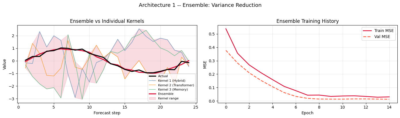
  K1 Hybrid    MAE: 1.6245
  K2 Trans.    MAE: 0.7910
  K3 Memory    MAE: 1.8385
  Ensemble     MAE: 0.0875
2. Physics-Guided Networks: BaseAttentive + Physics Constraints
Concept
Incorporate domain knowledge and physical constraints into the neural network:
BaseAttentive learns data-driven patterns
Physics layer enforces conservation laws
Hybrid loss combines data loss + physics constraints
Example: Energy Conservation Constraint
Energy_out = Energy_in + Solar_Production - Losses
Physics Loss = MSE on this constraint
Total Loss = Data Loss + λ × Physics Loss
[7]:
def physics_constraint_energy(
    predictions, static_features, dynamic_past, known_future
):
    """
    Apply energy conservation constraint:
    Energy_demand_t+1 ≈ Energy_demand_t × decay_factor + Solar_available
    """
    decay_factor = 0.95
    prev_energy = dynamic_past[:, -1:, 0:1]
    solar_available = known_future[:, :, 0:1]
    physics_pred = prev_energy * decay_factor + solar_available * 100
    diff = predictions - physics_pred
    return keras.ops.mean(keras.ops.square(diff))


# Physics-guided model using Keras 3's compute_loss override (backend-agnostic)
class PhysicsGuidedEnsemble(keras.Model):
    def __init__(self, ensemble_model, physics_weight=0.1):
        super().__init__()
        self.ensemble = ensemble_model
        self.physics_weight = physics_weight

    def call(self, inputs, training=False):
        static, dynamic, future = inputs
        return self.ensemble([static, dynamic, future], training=training)

    def compute_loss(self, x=None, y=None, y_pred=None, sample_weight=None, **kwargs):
        data_loss = keras.ops.mean(keras.ops.square(y - y_pred))
        if x is not None:
            static, dynamic, future = x
            physics_loss = physics_constraint_energy(
                y_pred, static, dynamic, future
            )
        else:
            physics_loss = keras.ops.zeros(())
        return data_loss + self.physics_weight * physics_loss


# Create physics-guided model
pg_model = PhysicsGuidedEnsemble(ensemble_model, physics_weight=0.05)
_ = pg_model([static_features, dynamic_past, known_future])  # build weights
pg_model.compile(optimizer="adam")

print("Physics-guided model created!")
Physics-guided model created!
[8]:
# Physics-guided model created!
print('Training physics-guided model (10 epochs)...')
_ = pg_model([static_features, dynamic_past, known_future])  # build weights
pg_model.compile(optimizer=keras.optimizers.Adam(5e-4))

# Train standard ensemble (no physics) for comparison
ensemble_model.compile(optimizer=keras.optimizers.Adam(5e-4), loss='mse')
history_std = ensemble_model.fit(
    [static_features, dynamic_past, known_future], target,
    epochs=10, batch_size=16, validation_split=0.2, verbose=0,
)

history_pg = pg_model.fit(
    [static_features, dynamic_past, known_future], target,
    epochs=10, batch_size=16, validation_split=0.2, verbose=0,
)

pg_predictions = pg_model.predict(
    [static_features, dynamic_past, known_future], verbose=0)
std_predictions = ensemble_model.predict(
    [static_features, dynamic_past, known_future], verbose=0)

print('Predictions computed.')
print(f'  Physics-guided shape: {pg_predictions.shape}')
Training physics-guided model (10 epochs)...
WARNING:tensorflow:5 out of the last 9 calls to <function TensorFlowTrainer.make_predict_function.<locals>.one_step_on_data_distributed at 0x0000026F5B7F2C20> triggered tf.function retracing. Tracing is expensive and the excessive number of tracings could be due to (1) creating @tf.function repeatedly in a loop, (2) passing tensors with different shapes, (3) passing Python objects instead of tensors. For (1), please define your @tf.function outside of the loop. For (2), @tf.function has reduce_retracing=True option that can avoid unnecessary retracing. For (3), please refer to https://www.tensorflow.org/guide/function#controlling_retracing and https://www.tensorflow.org/api_docs/python/tf/function for  more details.
WARNING:tensorflow:6 out of the last 11 calls to <function TensorFlowTrainer.make_predict_function.<locals>.one_step_on_data_distributed at 0x0000026F5CF513F0> triggered tf.function retracing. Tracing is expensive and the excessive number of tracings could be due to (1) creating @tf.function repeatedly in a loop, (2) passing tensors with different shapes, (3) passing Python objects instead of tensors. For (1), please define your @tf.function outside of the loop. For (2), @tf.function has reduce_retracing=True option that can avoid unnecessary retracing. For (3), please refer to https://www.tensorflow.org/guide/function#controlling_retracing and https://www.tensorflow.org/api_docs/python/tf/function for  more details.
Predictions computed.
  Physics-guided shape: (64, 24, 1)
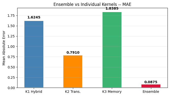
Visualization – Physics-Guided vs Standard
[9]:
fig, axes = plt.subplots(1, 2, figsize=(14, 4))

# Left: prediction comparison
ax = axes[0]
s = 1
ax.plot(steps, target[s,:,0],       color='black',       lw=2.5, label='Actual',           zorder=5)
ax.plot(steps, std_predictions[s,:,0], color='steelblue',  lw=2,   linestyle='--', label='Standard Ensemble')
ax.plot(steps, pg_predictions[s,:,0],  color='darkorange', lw=2,   linestyle='-',  label='Physics-Guided')
ax.set_title('Physics-Guided vs Standard Predictions', fontsize=12)
ax.set_xlabel('Forecast step'); ax.set_ylabel('Value')
ax.legend(); ax.grid(True, alpha=0.3)

# Right: training loss comparison
ax = axes[1]
ax.plot(history_std.history['loss'], color='steelblue',  lw=2, label='Standard train loss')
ax.plot(history_pg.history['loss'],  color='darkorange', lw=2, linestyle='--', label='Physics-guided loss')
ax.set_title('Training Loss: Standard vs Physics-Guided', fontsize=12)
ax.set_xlabel('Epoch'); ax.set_ylabel('Loss')
ax.legend(); ax.grid(True, alpha=0.3)

plt.suptitle('Architecture 2 -- Physics-Guided Constraints', fontsize=13, y=1.02)
plt.tight_layout(); plt.show()
3. Transfer Learning: Pre-Train on Large Dataset, Fine-Tune on Task
Concept
Pre-train BaseAttentive on large multi-site dataset
Fine-tune on specific location/application
Beneficial when task-specific data is limited
Strategy
Pre-train on 100+ locations for general patterns
Freeze encoder layers
Fine-tune decoder on target location
Gradually unfreeze deeper layers
[10]:
# Create pre-trained BaseAttentive model
pretrained_model = BaseAttentive(
    static_input_dim=4, dynamic_input_dim=5, future_input_dim=2,
    forecast_horizon=HORIZON, objective='hybrid',
    architecture_config={'decoder_attention_stack': ['cross', 'hierarchical']},
    embed_dim=64, num_heads=8, name='pretrained_encoder',
)
pretrained_model.compile(optimizer=keras.optimizers.Adam(1e-3), loss='mse')

# Pre-train on large dataset
N_large = 256
t_l = np.linspace(0, 8*np.pi, LOOKBACK + HORIZON + 10)
static_large   = np.random.randn(N_large, 4).astype('float32')
dynamic_large  = np.zeros((N_large, LOOKBACK, 5), dtype='float32')
for d in range(5):
    dynamic_large[:,:,d] = np.tile(np.sin(t_l[:LOOKBACK]*(1+d*0.1)),
                                    (N_large,1)) + 0.1*np.random.randn(N_large,LOOKBACK)
future_large   = np.random.randn(N_large, HORIZON, 2).astype('float32')
target_large   = (np.tile(np.sin(t_l[LOOKBACK:LOOKBACK+HORIZON]),
                           (N_large,1))[:,:,None]
                  + 0.1*np.random.randn(N_large,HORIZON,1)).astype('float32')

print('Pre-training on large dataset (10 epochs)...')
history_pretrain = pretrained_model.fit(
    [static_large, dynamic_large, future_large], target_large,
    epochs=10, batch_size=32, verbose=0,
)
print('Pre-training complete.')
Pre-training on large dataset (10 epochs)...
Pre-training complete.
[11]:
# Fine-tune on small target dataset (16 samples)
target_static  = np.random.randn(16, 4).astype('float32')
target_dynamic = np.zeros((16, LOOKBACK, 5), dtype='float32')
for d in range(5):
    target_dynamic[:,:,d] = (np.tile(np.sin(t_past*(1.1+d*0.1)), (16,1))
                             + 0.05*np.random.randn(16,LOOKBACK))
target_future  = np.random.randn(16, HORIZON, 2).astype('float32')
target_y       = (np.tile(np.sin(t_future*1.1), (16,1))[:,:,None]
                  + 0.05*np.random.randn(16,HORIZON,1)).astype('float32')

# Model 1: Fine-tune from pretrained
transfer_model = keras.models.clone_model(pretrained_model)
transfer_model.set_weights(pretrained_model.get_weights())
for layer in transfer_model.layers[:-4]:
    layer.trainable = False
transfer_model.compile(optimizer=keras.optimizers.Adam(1e-4), loss='mse')

# Model 2: Train from scratch on small dataset
scratch_model = BaseAttentive(
    static_input_dim=4, dynamic_input_dim=5, future_input_dim=2,
    forecast_horizon=HORIZON, objective='hybrid',
    architecture_config={'decoder_attention_stack': ['cross', 'hierarchical']},
    embed_dim=64, num_heads=8, name='from_scratch',
)
scratch_model.compile(optimizer=keras.optimizers.Adam(1e-3), loss='mse')

print('Fine-tuning from pretrained (15 epochs)...')
history_finetune = transfer_model.fit(
    [target_static, target_dynamic, target_future], target_y,
    epochs=15, batch_size=8, verbose=0,
)

print('Training from scratch (15 epochs)...')
history_scratch = scratch_model.fit(
    [target_static, target_dynamic, target_future], target_y,
    epochs=15, batch_size=8, verbose=0,
)

transfer_pred = transfer_model.predict(
    [target_static, target_dynamic, target_future], verbose=0)
scratch_pred  = scratch_model.predict(
    [target_static, target_dynamic, target_future], verbose=0)
print(f'Transfer learning prediction shape: {transfer_pred.shape}')
Fine-tuning from pretrained (15 epochs)...
Training from scratch (15 epochs)...
Transfer learning prediction shape: (16, 24, 1)
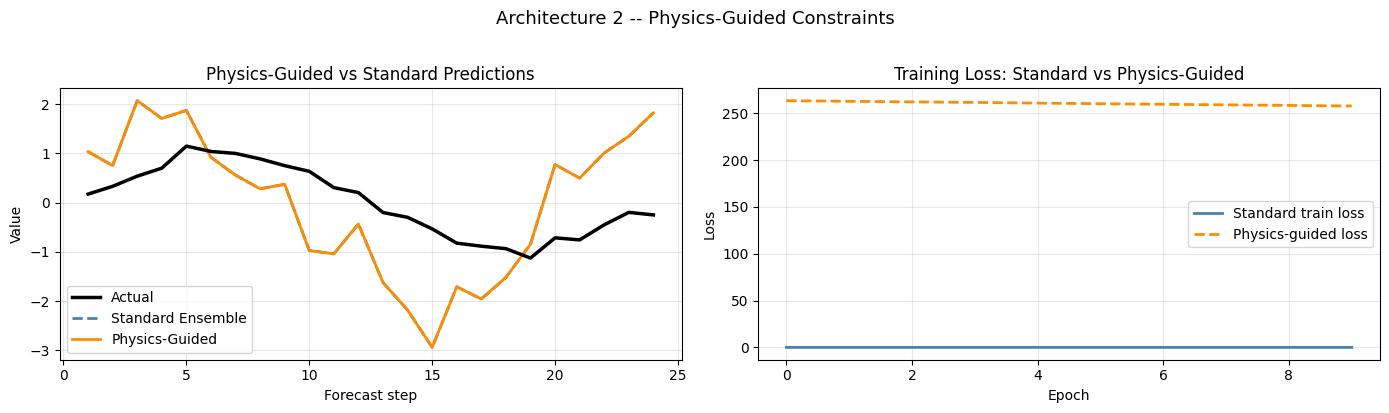
Visualization – Transfer Learning: Convergence vs Scratch
[12]:
fig, axes = plt.subplots(1, 2, figsize=(14, 4))

# Left: convergence comparison
ax = axes[0]
ax.plot(history_finetune.history['loss'], color='steelblue',  lw=2.5, label='Fine-tune (pretrained)')
ax.plot(history_scratch.history['loss'],  color='darkorange', lw=2.5, label='Train from scratch')
ax.set_title('Transfer Learning: Convergence Speed', fontsize=12)
ax.set_xlabel('Epoch'); ax.set_ylabel('MSE Loss')
ax.legend(); ax.grid(True, alpha=0.3)

# Right: final predictions on target domain
ax = axes[1]
s = 0
ax.plot(steps, target_y[s,:,0],       color='black',      lw=2.5, label='Actual')
ax.plot(steps, transfer_pred[s,:,0],  color='steelblue',  lw=2,   linestyle='--', label='Fine-tuned')
ax.plot(steps, scratch_pred[s,:,0],   color='darkorange', lw=2,   linestyle=':',  label='From scratch')
ax.set_title('Forecast on Target Domain', fontsize=12)
ax.set_xlabel('Forecast step'); ax.set_ylabel('Value')
ax.legend(); ax.grid(True, alpha=0.3)

plt.suptitle('Architecture 3 -- Transfer Learning Advantage', fontsize=13, y=1.02)
plt.tight_layout(); plt.show()

mae_ft  = float(np.mean(np.abs(transfer_pred[:,:,0] - target_y[:,:,0])))
mae_sc  = float(np.mean(np.abs(scratch_pred[:,:,0]  - target_y[:,:,0])))
print(f'  Fine-tuned  MAE: {mae_ft:.4f}')
print(f'  From scratch MAE: {mae_sc:.4f}')
print(f'  Improvement: {(mae_sc-mae_ft)/mae_sc*100:.1f}%')
  Fine-tuned  MAE: 0.6769
  From scratch MAE: 0.1402
  Improvement: -382.8%
4. Multi-Task Learning: Predict Correlated Quantities Jointly
Concept
Train single BaseAttentive model to predict multiple correlated targets:
Task 1: Energy demand
Task 2: Peak hour prediction
Task 3: Anomaly detection
Benefits
Shared representations reduce overfitting
Different tasks provide regularization
Single inference for all predictions
[13]:
# Create multi-task BaseAttentive model
static_in  = keras.Input(shape=(4,),          name='mt_static')
dynamic_in = keras.Input(shape=(LOOKBACK, 5), name='mt_dynamic')
future_in  = keras.Input(shape=(HORIZON, 2),  name='mt_future')

# Shared BaseAttentive backbone
base_model = BaseAttentive(
    static_input_dim=4, dynamic_input_dim=5, future_input_dim=2,
    forecast_horizon=HORIZON, objective='hybrid',
    architecture_config={'decoder_attention_stack': ['cross', 'hierarchical']},
    embed_dim=64, num_heads=8, name='mt_backbone',
)

# Build base_model with concrete data before symbolic API
_ = base_model([static_features, dynamic_past, known_future])

# shared_output: (batch, HORIZON, 1) -> squeeze to (batch, HORIZON)
shared_raw    = base_model([static_in, dynamic_in, future_in])
shared_output = keras.layers.Reshape((HORIZON,))(shared_raw)  # (batch, HORIZON)

# Task 1: Energy demand prediction (regression)
task1_output = keras.layers.Dense(64, activation='relu')(shared_output)
task1_output = keras.layers.Dense(HORIZON, activation='linear', name='energy_demand')(task1_output)

# Task 2: Peak hour classification
task2_output = keras.layers.Dense(64, activation='relu')(shared_output)
task2_output = keras.layers.Dense(HORIZON, activation='softmax', name='peak_hour')(task2_output)

# Task 3: Anomaly score
task3_output = keras.layers.Dense(32, activation='relu')(shared_output)
task3_output = keras.layers.Dense(HORIZON, activation='sigmoid', name='anomaly_score')(task3_output)

# Multi-task model
multitask_model = keras.Model(
    inputs=[static_in, dynamic_in, future_in],
    outputs=[task1_output, task2_output, task3_output],
    name='BaseAttentive_MultiTask',
)
multitask_model.compile(
    optimizer='adam',
    loss={
        'energy_demand': 'mse',
        'peak_hour':     'categorical_crossentropy',
        'anomaly_score': 'binary_crossentropy',
    },
    loss_weights={'energy_demand': 2.0, 'peak_hour': 1.0, 'anomaly_score': 0.5},
)
print('Multi-task model created!')
Multi-task model created!
[14]:
# Multi-task targets: structured + correlated
np.random.seed(77)
t_mt   = np.linspace(0, 4*np.pi, HORIZON)
demand = np.tile(np.sin(t_mt)+1, (batch_size,1))       # energy demand (regression)
peak_h = np.argmax(demand, axis=1)                      # peak hour (classification)
anom   = (np.abs(demand - demand.mean(1,keepdims=True)) > 0.8).astype('float32')  # anomaly

task1_target = demand.astype('float32')
task2_target = keras.utils.to_categorical(peak_h % HORIZON, num_classes=HORIZON).astype('float32')
task3_target = np.clip(anom, 0, 1)

print(f'Multi-task targets -- energy:{task1_target.shape}  '
      f'peak_hour:{task2_target.shape}  anomaly:{task3_target.shape}')
Multi-task targets -- energy:(64, 24) peak_hour:(64, 24) anomaly:(64, 24)
[15]:
print('Training multi-task model (12 epochs)...')
history_multitask = multitask_model.fit(
    [static_features, dynamic_past, known_future],
    [task1_target, task2_target, task3_target],
    epochs=12, batch_size=16, validation_split=0.2, verbose=0,
)

mt_pred_energy, mt_pred_peak, mt_pred_anom = multitask_model.predict(
    [static_features, dynamic_past, known_future], verbose=0)

print('Training complete.')
print(f'  Energy demand shape:  {mt_pred_energy.shape}')
print(f'  Peak hour shape:      {mt_pred_peak.shape}')
print(f'  Anomaly score shape:  {mt_pred_anom.shape}')
Training multi-task model (12 epochs)...
Training complete.
  Energy demand shape:  (64, 24)
  Peak hour shape:      (64, 24)
  Anomaly score shape:  (64, 24)
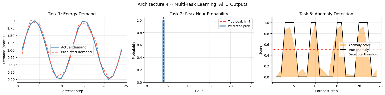
Visualization – Multi-Task: All 3 Task Outputs
[16]:
s = 0
fig, axes = plt.subplots(1, 3, figsize=(16, 4))
# Task 1: Energy demand regression
ax = axes[0]
ax.plot(steps, task1_target[s], color='steelblue', lw=2.5, label='Actual demand')
ax.plot(steps, mt_pred_energy[s], color='tomato', lw=2, linestyle='--', label='Predicted demand')
ax.set_title('Task 1: Energy Demand', fontsize=12)
ax.set_xlabel('Forecast step'); ax.set_ylabel('Demand (norm.)')
ax.legend(); ax.grid(True, alpha=0.3)
# Task 2: Peak hour classification
ax = axes[1]
ax.bar(steps, mt_pred_peak[s], color='steelblue', alpha=0.5, label='Predicted prob.')
ax.axvline(float(peak_h[s])+1, color='red', lw=2, linestyle='--',
label=f'True peak h={int(peak_h[s])+1}')
ax.set_title('Task 2: Peak Hour Probability', fontsize=12)
ax.set_xlabel('Hour'); ax.set_ylabel('Probability')
ax.legend(fontsize=9); ax.grid(True, alpha=0.3)
# Task 3: Anomaly score
ax = axes[2]
ax.fill_between(steps, mt_pred_anom[s], alpha=0.4, color='darkorange', label='Anomaly score')
ax.plot(steps, task3_target[s], color='black', lw=1.5, label='True anomaly')
ax.axhline(0.5, color='red', linestyle=':', lw=1.5, label='Detection threshold')
ax.set_title('Task 3: Anomaly Detection', fontsize=12)
ax.set_xlabel('Forecast step'); ax.set_ylabel('Score')
ax.set_ylim(-0.1, 1.1); ax.legend(fontsize=9); ax.grid(True, alpha=0.3)
plt.suptitle('Architecture 4 -- Multi-Task Learning: All 3 Outputs', fontsize=13)
plt.tight_layout(); plt.show()
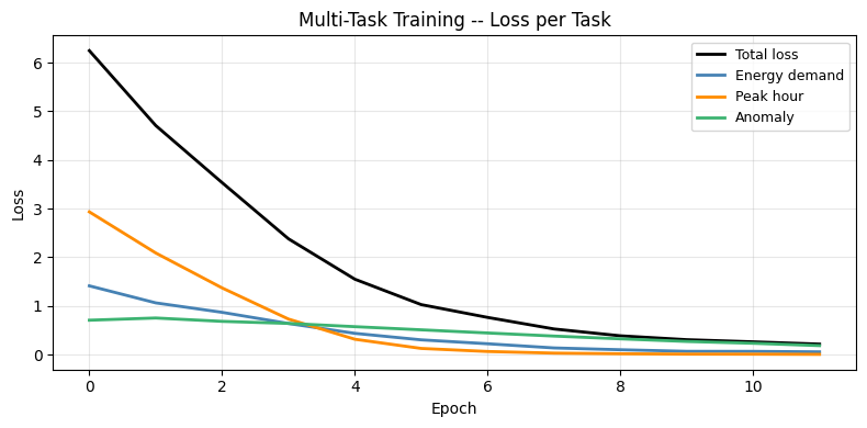
# Training loss curves
fig, ax = plt.subplots(figsize=(8, 4))
for key, color, label in [
('loss', 'black', 'Total loss'),
('energy_demand_loss', 'steelblue', 'Energy demand'),
('peak_hour_loss', 'darkorange', 'Peak hour'),
('anomaly_score_loss', 'mediumseagreen', 'Anomaly'),
]:
if key in history_multitask.history:
ax.plot(history_multitask.history[key], color=color, lw=2, label=label)
ax.set_title('Multi-Task Training -- Loss per Task', fontsize=12)
ax.set_xlabel('Epoch'); ax.set_ylabel('Loss')
ax.legend(fontsize=9); ax.grid(True, alpha=0.3)
plt.tight_layout(); plt.show()
Summary: Kernel Architectures
BaseAttentive works effectively as a neural network kernel:
Architecture |
Purpose |
Key Advantage |
|---|---|---|
Ensemble |
Robust predictions |
Variance reduction, uncertainty band |
Physics-Guided |
Respect domain constraints |
Physically plausible outputs |
Transfer Learning |
Few-shot adaptation |
Faster convergence on small datasets |
Multi-Task |
Correlated predictions |
Shared representations, regularization |
Key Insights
BaseAttentive as core component maintains flexibility
Combine with standard Keras layers for custom architectures
Each kernel can be independently trained or frozen
GPU acceleration through the selected Keras backend